Functionality for classical multidimensional scaling objects
Source:R/methods-stats-cmds.r
methods-cmds.RdThese methods extract data from, and attribute new data to,
objects of class "cmds_ord". This is a class introduced in this package
to identify objects returned by cmdscale_ord(), which wraps
stats::cmdscale().
Usage
# S3 method for class 'cmds_ord'
as_tbl_ord(x)

# S3 method for class 'cmds_ord'
recover_rows(x)

# S3 method for class 'cmds_ord'
recover_cols(x)

# S3 method for class 'cmds_ord'
recover_inertia(x)

# S3 method for class 'cmds_ord'
recover_coord(x)

# S3 method for class 'cmds_ord'
recover_conference(x)

# S3 method for class 'cmds_ord'
recover_aug_rows(x)

# S3 method for class 'cmds_ord'
recover_aug_cols(x)

# S3 method for class 'cmds_ord'
recover_aug_coord(x)Value
The recovery generics recover_*() return core model components, distribution of inertia,
supplementary elements, and intrinsic metadata; but they require methods for each model class to
tell them what these components are.
The generic as_tbl_ord() returns its input wrapped in the 'tbl_ord'
class. Its methods determine what model classes it is allowed to wrap. It
then provides 'tbl_ord' methods with access to the recoverers and hence to
the model components.
See also
Other methods for eigen-decomposition-based techniques:
methods-eigen,
methods-factanal,
methods-princomp
Other models from the stats package:
methods-cancor,
methods-factanal,
methods-kmeans,
methods-lm,
methods-prcomp,
methods-princomp
Examples
# 'dist' object (matrix of road distances) of large American cities
class(UScitiesD)
#> [1] "dist"
print(UScitiesD)
#>               Atlanta Chicago Denver Houston LosAngeles Miami NewYork
#> Chicago           587
#> Denver           1212     920
#> Houston           701     940    879
#> LosAngeles       1936    1745    831    1374
#> Miami             604    1188   1726     968       2339
#> NewYork           748     713   1631    1420       2451  1092
#> SanFrancisco     2139    1858    949    1645        347  2594    2571
#> Seattle          2182    1737   1021    1891        959  2734    2408
#> Washington.DC     543     597   1494    1220       2300   923     205
#>               SanFrancisco Seattle
#> Chicago
#> Denver
#> Houston
#> LosAngeles
#> Miami
#> NewYork
#> SanFrancisco
#> Seattle                678
#> Washington.DC         2442    2329

# use multidimensional scaling to infer artificial planar coordinates
UScitiesD %>%
  cmdscale_ord(k = 2) %>%
  as_tbl_ord() %>%
  print() -> usa_mds
#> # A tbl_ord of class 'cmds_ord': (10 × 2) · (0 × 2)´
#> # 2 coordinates: PCo1 and PCo2
#> # Rows (principal, 100%): [ 10 × 2 | 0 ]
#>      PCo1   PCo2 |
#> [9.2e+13][3e+12] |
#>  1  -719.  143.  |
#>  2  -382. -341.  |
#>  3   482.  -25.3 |
#>  4  -161.  573.  |
#>  5  1204.  390.  |
#>  6 -1134.  582.  |
#>  7 -1072. -519.  |
#>  8  1421.  113.  |
#>  9  1342. -580.  |
#> 10  -980. -335.  |
#> # Columns (standard, 0%): [ 0 × 2 | 0 ]
#>      PCo1   PCo2 |
#>     <dbl>  <dbl> |

# recover (equivalent) matrices of row and column artificial coordinates
get_rows(usa_mds)
#>                     PCo1       PCo2
#> Atlanta        -718.7594  142.99427
#> Chicago        -382.0558 -340.83962
#> Denver          481.6023  -25.28504
#> Houston        -161.4663  572.76991
#> LosAngeles     1203.7380  390.10029
#> Miami         -1133.5271  581.90731
#> NewYork       -1072.2357 -519.02423
#> SanFrancisco   1420.6033  112.58920
#> Seattle        1341.7225 -579.73928
#> Washington.DC  -979.6220 -335.47281
get_cols(usa_mds)
#>      PCo1 PCo2

# augment ordination with point names
(usa_mds <- augment_ord(usa_mds))
#> # A tbl_ord of class 'cmds_ord': (10 × 2) · (0 × 2)´
#> # 2 coordinates: PCo1 and PCo2
#> # Rows (principal, 100%): [ 10 × 2 | 2 ]
#>      PCo1   PCo2 | name          .element
#> [9.2e+13][3e+12] | <chr>         <chr>
#>  1  -719.  143.  | Atlanta       active
#>  2  -382. -341.  | Chicago       active
#>  3   482.  -25.3 | Denver        active
#>  4  -161.  573.  | Houston       active
#>  5  1204.  390.  | LosAngeles    active
#>  6 -1134.  582.  | Miami         active
#>  7 -1072. -519.  | NewYork       active
#>  8  1421.  113.  | SanFrancisco  active
#>  9  1342. -580.  | Seattle       active
#> 10  -980. -335.  | Washington.DC active
#> # Columns (standard, 0%): [ 0 × 2 | 1 ]
#>      PCo1   PCo2 |
#>     <dbl>  <dbl> |

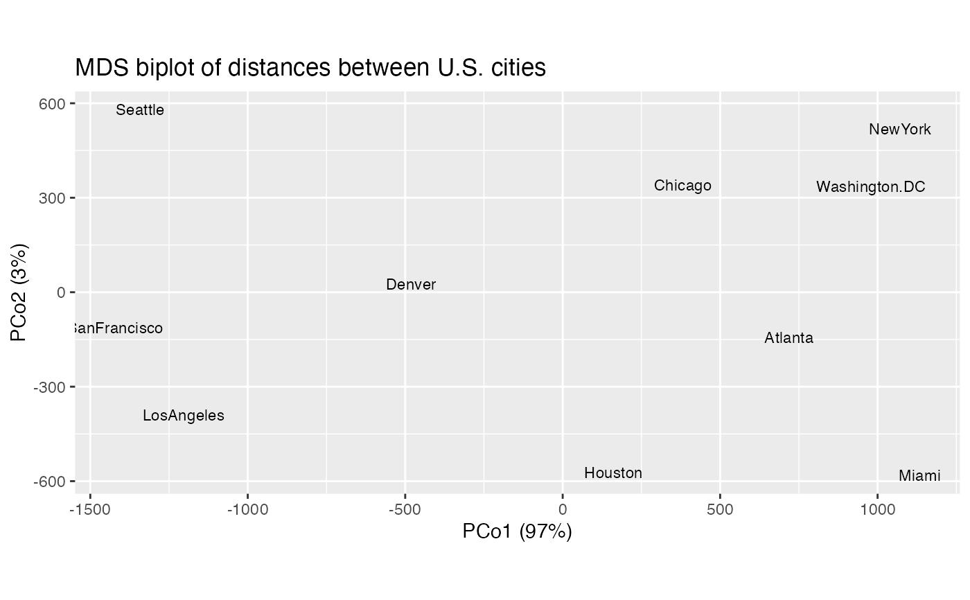
# reorient biplot to conventional compass
usa_mds %>%
  negate_ord(c(1, 2)) %>%
  ggbiplot() +
  geom_cols_text(aes(label = name), size = 3) +
  ggtitle("MDS biplot of distances between U.S. cities")