Functionality for factor analysis ('factanal') objects
Source:R/methods-stats-factanal.r
methods-factanal.RdThese methods extract data from, and attribute new data to,
objects of class "factanal" as returned by stats::factanal().
Usage
# S3 method for class 'factanal'
as_tbl_ord(x)

# S3 method for class 'factanal'
recover_rows(x)

# S3 method for class 'factanal'
recover_cols(x)

# S3 method for class 'factanal'
recover_inertia(x)

# S3 method for class 'factanal'
recover_coord(x)

# S3 method for class 'factanal'
recover_conference(x)

# S3 method for class 'factanal'
recover_supp_rows(x)

# S3 method for class 'factanal'
recover_aug_rows(x)

# S3 method for class 'factanal'
recover_aug_cols(x)

# S3 method for class 'factanal'
recover_aug_coord(x)Value
The recovery generics recover_*() return core model components, distribution of inertia,
supplementary elements, and intrinsic metadata; but they require methods for each model class to
tell them what these components are.
The generic as_tbl_ord() returns its input wrapped in the 'tbl_ord'
class. Its methods determine what model classes it is allowed to wrap. It
then provides 'tbl_ord' methods with access to the recoverers and hence to
the model components.
Details
Factor analysis of a data matrix relies on an an eigendecomposition of its
correlation matrix, whose eigenvectors (up to weighting) comprise the
variable loadings. For this reason, both row and column recoverers retrieve
the loadings and inertia is evenly distributed between them. When computed
and returned by stats::factanal(), the case scores are accessible as
supplementary elements. Redistribution of inertia commutes through both
score calculations.
See also
Other methods for eigen-decomposition-based techniques:
methods-cmds,
methods-eigen,
methods-princomp
Other models from the stats package:
methods-cancor,
methods-cmds,
methods-kmeans,
methods-lm,
methods-prcomp,
methods-princomp
Examples
# data frame of Swiss fertility and socioeconomic indicators
class(swiss)
#> [1] "data.frame"
head(swiss)
#>              Fertility Agriculture Examination Education Catholic
#> Courtelary        80.2        17.0          15        12     9.96
#> Delemont          83.1        45.1           6         9    84.84
#> Franches-Mnt      92.5        39.7           5         5    93.40
#> Moutier           85.8        36.5          12         7    33.77
#> Neuveville        76.9        43.5          17        15     5.16
#> Porrentruy        76.1        35.3           9         7    90.57
#>              Infant.Mortality
#> Courtelary               22.2
#> Delemont                 22.2
#> Franches-Mnt             20.2
#> Moutier                  20.3
#> Neuveville               20.6
#> Porrentruy               26.6
# perform factor analysis
swiss_fa <- factanal(~ ., factors = 2L, data = swiss, scores = "regression")

# wrap as a 'tbl_ord' object
(swiss_fa <- as_tbl_ord(swiss_fa))
#> # A tbl_ord of class 'factanal': (47 x 2) x (6 x 2)'
#> # 2 coordinates: Factor1 and Factor2
#> #
#> # Rows (principal): [ 47 x 2 | 0 ]
#>   Factor1 Factor2 |
#>                   |
#> 1  0.0791  -0.634 |
#> 2 -0.179    1.08  |
#> 3 -0.588    1.20  |
#> 4 -0.424   -0.158 |
#> 5  0.382   -0.668 |
#> # ℹ 42 more rows |
#>
#> #
#> # Columns (principal): [ 6 x 2 | 0 ]
#>   Factor1 Factor2 |
#>                   |
#> 1 -0.652   0.393  |
#> 2 -0.631   0.333  |
#> 3  0.685  -0.510  |
#> 4  0.997  -0.0313 |
#> 5 -0.124   0.961  |
#> 6 -0.0947  0.175  |

# recover loadings
get_rows(swiss_fa, elements = "active")
#>      Factor1 Factor2
get_cols(swiss_fa)
#>                      Factor1     Factor2
#> Fertility        -0.65238512  0.39335226
#> Agriculture      -0.63054439  0.33275063
#> Examination       0.68498141 -0.51036433
#> Education         0.99700850 -0.03128268
#> Catholic         -0.12417831  0.96118093
#> Infant.Mortality -0.09466294  0.17483734
# recover scores
head(get_rows(swiss_fa, elements = "score"))
#>                  Factor1    Factor2
#> Courtelary    0.07912746 -0.6344915
#> Delemont     -0.17926953  1.0783941
#> Franches-Mnt -0.58784929  1.2004233
#> Moutier      -0.42433417 -0.1583409
#> Neuveville    0.38211185 -0.6682790
#> Porrentruy   -0.37286722  1.0884740

# augment column loadings with uniquenesses
(swiss_fa <- augment_ord(swiss_fa))
#> # A tbl_ord of class 'factanal': (47 x 2) x (6 x 2)'
#> # 2 coordinates: Factor1 and Factor2
#> #
#> # Rows (principal): [ 47 x 2 | 2 ]
#>   Factor1 Factor2 |   .element name
#>                   |   <chr>    <chr>
#> 1  0.0791  -0.634 | 1 score    Courtelary
#> 2 -0.179    1.08  | 2 score    Delemont
#> 3 -0.588    1.20  | 3 score    Franches-Mnt
#> 4 -0.424   -0.158 | 4 score    Moutier
#> 5  0.382   -0.668 | 5 score    Neuveville
#> # ℹ 42 more rows | # ℹ 42 more rows
#>
#> #
#> # Columns (principal): [ 6 x 2 | 3 ]
#>   Factor1 Factor2 |   name           uniqueness .element
#>                   |   <chr>               <dbl> <chr>
#> 1 -0.652   0.393  | 1 Fertility          0.420  active
#> 2 -0.631   0.333  | 2 Agriculture        0.492  active
#> 3  0.685  -0.510  | 3 Examination        0.270  active
#> 4  0.997  -0.0313 | 4 Education          0.005  active
#> 5 -0.124   0.961  | 5 Catholic           0.0607 active
#> 6 -0.0947  0.175  | 6 Infant.Mortal…     0.960  active

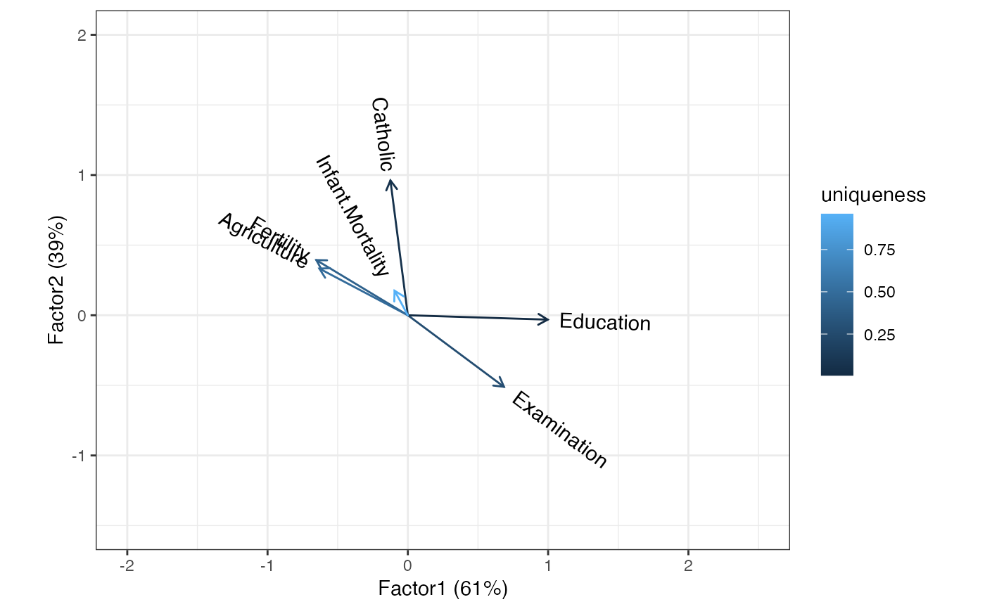
# symmetric biplot
swiss_fa %>%
  ggbiplot() +
  theme_bw() +
  geom_cols_vector(aes(color = uniqueness, label = name)) +
  expand_limits(x = c(-2, 2.5), y = c(-1.5, 2))
