ordr integrates ordination analysis and biplot visualization into Tidyverse workflows.
motivation
Wherever there is an SVD, there is a biplot.1
ordination and biplots
Ordination is a catch-all term for a variety of statistical techniques that introduce an artificial coordinate system for a data set in such a way that a few coordinates capture a large amount of the data structure 2. The branch of mathematical statistics called geometric data analysis (GDA) provides the theoretical basis for (most of) these techniques. Ordination overlaps with regression and with dimension reduction, which can be contrasted to clustering and classification in that they assign continuous rather than categorical values to data elements 3.
Most ordination techniques decompose a numeric rectangular data set into the product of two matrices, often using singular value decomposition (SVD). The coordinates of the shared dimensions of these matrices (over which they are multiplied) are the artificial coordinates. In some cases, such as principal components analysis, the decomposition is exact; in others, such as non-negative matrix factorization, it is approximate. Some techniques, such as correspondence analysis, transform the data before decomposition. Ordination techniques may be supervised, like linear discriminant analysis, or unsupervised, like multidimensional scaling.
Analysis pipelines that use these techniques may use the artificial coordinates directly, in place of natural coordinates, to arrange and compare data elements or to predict responses. This is possible because both the rows and the columns of the original table can be located, or positioned, along these shared coordinates. The number of artificial coordinates used in an application, such as regression or visualization, is called the rank of the ordination 4. A common application is the biplot, which positions the rows and columns of the original table in a scatterplot in 1, 2, or 3 artificial coordinates, usually those that explain the most variation in the data.
implementations in R
An extensive range of ordination techniques are implemented in R, from classical multidimensional scaling (stats::cmdscale()) and principal components analysis (stats::prcomp() and stats::princomp()) in the stats package distributed with base R, across widely-used implementations of linear discriminant analysis (MASS::lda()) and correspondence analysis (ca::ca()) in general-use statistical packages, to highly specialized packages that implement cutting-edge techniques or adapt conventional techniques to challenging settings. These implementations come with their own conventions, tailored to the research communities that produced them, and it would be impractical (and probably unhelpful) to try to consolidate them.
Instead, ordr provides a streamlined process by which the models output by these methods—in particular, the matrix factors into which the original data are approximately decomposed and the artificial coordinates they share—can be inspected, annotated, tabulated, summarized, and visualized. On this last point, most biplot implementations in R provide limited customizability. ordr adopts the grammar of graphics paradigm from ggplot2 to modularize and standardize biplot elements 5. Overall, the package is designed to follow the broader syntactic conventions of the Tidyverse, so that users familiar with a this workflow can more easily and quickly integrate ordination models into practice.
usage
installation
ordr is now on CRAN and can be installed using base R:
install.packages("ordr")The development version can be installed from the (default) main branch using remotes:
remotes::install_github("corybrunson/ordr")example
Morphologically, Iris versicolor is much closer to Iris virginica than to Iris setosa, though in every character by which it differs from Iris virginica it departs in the direction of Iris setosa.6
A very common illustration of ordination in R applies principal components analysis (PCA) to Anderson’s iris measurements. These data consist of lengths and widths of the petals and surrounding sepals from 50 each of three species of iris:
head(iris)
#>   Sepal.Length Sepal.Width Petal.Length Petal.Width Species
#> 1          5.1         3.5          1.4         0.2  setosa
#> 2          4.9         3.0          1.4         0.2  setosa
#> 3          4.7         3.2          1.3         0.2  setosa
#> 4          4.6         3.1          1.5         0.2  setosa
#> 5          5.0         3.6          1.4         0.2  setosa
#> 6          5.4         3.9          1.7         0.4  setosa
summary(iris)
#>   Sepal.Length    Sepal.Width     Petal.Length    Petal.Width
#>  Min.   :4.300   Min.   :2.000   Min.   :1.000   Min.   :0.100
#>  1st Qu.:5.100   1st Qu.:2.800   1st Qu.:1.600   1st Qu.:0.300
#>  Median :5.800   Median :3.000   Median :4.350   Median :1.300
#>  Mean   :5.843   Mean   :3.057   Mean   :3.758   Mean   :1.199
#>  3rd Qu.:6.400   3rd Qu.:3.300   3rd Qu.:5.100   3rd Qu.:1.800
#>  Max.   :7.900   Max.   :4.400   Max.   :6.900   Max.   :2.500
#>        Species
#>  setosa    :50
#>  versicolor:50
#>  virginica :50
#>
#>
#>
ordr provides a convenience function to send a subset of columns to an ordination function, wrap the resulting model in the tibble-derived ‘tbl_ord’ class, and append both model diagnostics and other original data columns as annotations to the appropriate matrix factors:7
library(ordr)
#> Loading required package: ggplot2
(iris_pca <- ordinate(iris, cols = 1:4, model = ~ prcomp(., scale. = TRUE)))
#> # A tbl_ord of class 'prcomp': (150 x 4) x (4 x 4)'
#> # 4 coordinates: PC1, PC2, ..., PC4
#> #
#> # Rows (principal): [ 150 x 4 | 1 ]
#>     PC1    PC2     PC3 ... |   Species
#>                            |   <fct>
#> 1 -2.26 -0.478  0.127      | 1 setosa
#> 2 -2.07  0.672  0.234      | 2 setosa
#> 3 -2.36  0.341 -0.0441 ... | 3 setosa
#> 4 -2.29  0.595 -0.0910     | 4 setosa
#> 5 -2.38 -0.645 -0.0157     | 5 setosa
#> # ℹ 145 more rows     | # ℹ 145 more rows
#>
#> #
#> # Columns (standard): [ 4 x 4 | 3 ]
#>      PC1     PC2    PC3 ... |   name         center scale
#>                             |   <chr>         <dbl> <dbl>
#> 1  0.521 -0.377   0.720     | 1 Sepal.Length   5.84 0.828
#> 2 -0.269 -0.923  -0.244 ... | 2 Sepal.Width    3.06 0.436
#> 3  0.580 -0.0245 -0.142     | 3 Petal.Length   3.76 1.77
#> 4  0.565 -0.0669 -0.634     | 4 Petal.Width    1.20 0.762
Additional annotations can be added using several row- and column-specific dplyr-style verbs:
iris_meta <- data.frame(
  Species = c("setosa", "versicolor", "virginica"),
  Colony = c(1L, 1L, 2L),
  Cytotype = c("diploid", "hexaploid", "tetraploid")
)
(iris_pca <- left_join_rows(iris_pca, iris_meta, by = "Species"))
#> # A tbl_ord of class 'prcomp': (150 x 4) x (4 x 4)'
#> # 4 coordinates: PC1, PC2, ..., PC4
#> #
#> # Rows (principal): [ 150 x 4 | 3 ]
#>     PC1    PC2     PC3 ... |   Species Colony Cytotype
#>                            |   <chr>    <int> <chr>
#> 1 -2.26 -0.478  0.127      | 1 setosa       1 diploid
#> 2 -2.07  0.672  0.234      | 2 setosa       1 diploid
#> 3 -2.36  0.341 -0.0441 ... | 3 setosa       1 diploid
#> 4 -2.29  0.595 -0.0910     | 4 setosa       1 diploid
#> 5 -2.38 -0.645 -0.0157     | 5 setosa       1 diploid
#> # ℹ 145 more rows     | # ℹ 145 more rows
#>
#> #
#> # Columns (standard): [ 4 x 4 | 3 ]
#>      PC1     PC2    PC3 ... |   name         center scale
#>                             |   <chr>         <dbl> <dbl>
#> 1  0.521 -0.377   0.720     | 1 Sepal.Length   5.84 0.828
#> 2 -0.269 -0.923  -0.244 ... | 2 Sepal.Width    3.06 0.436
#> 3  0.580 -0.0245 -0.142     | 3 Petal.Length   3.76 1.77
#> 4  0.565 -0.0669 -0.634     | 4 Petal.Width    1.20 0.762
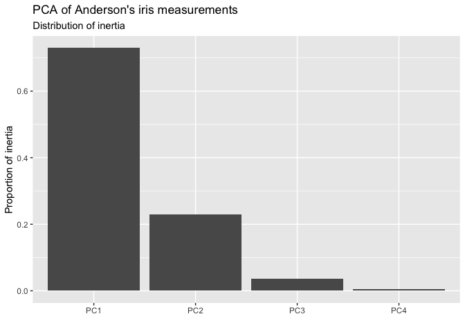
Following the broom package, the tidy() method produces a tibble describing the model components, in this case the principal coordinates, which is suitable for scree plotting:
tidy(iris_pca) %T>% print() %>%
  ggplot(aes(x = name, y = prop_var)) +
  geom_col() +
  labs(x = "", y = "Proportion of inertia") +
  ggtitle("PCA of Anderson's iris measurements",
          "Distribution of inertia")
#> # A tibble: 4 × 5
#>   name   sdev inertia prop_var quality
#>   <fct> <dbl>   <dbl>    <dbl>   <dbl>
#> 1 PC1   1.71   435.    0.730     0.730
#> 2 PC2   0.956  136.    0.229     0.958
#> 3 PC3   0.383   21.9   0.0367    0.995
#> 4 PC4   0.144    3.09  0.00518   1
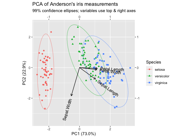
Following ggplot2, the fortify() method row-binds the factor tibbles with an additional .matrix column. This is used by ggbiplot() to redirect row- and column-specific plot layers to the appropriate subsets:8
ggbiplot(iris_pca, sec.axes = "cols", scale.factor = 2) +
  geom_rows_point(aes(color = Species, shape = Species)) +
  stat_rows_ellipse(aes(color = Species), alpha = .5, level = .99) +
  geom_cols_vector(aes(label = name)) +
  expand_limits(y = c(-3.5, NA)) +
  ggtitle("PCA of Anderson's iris measurements",
          "99% confidence ellipses; variables use top & right axes")
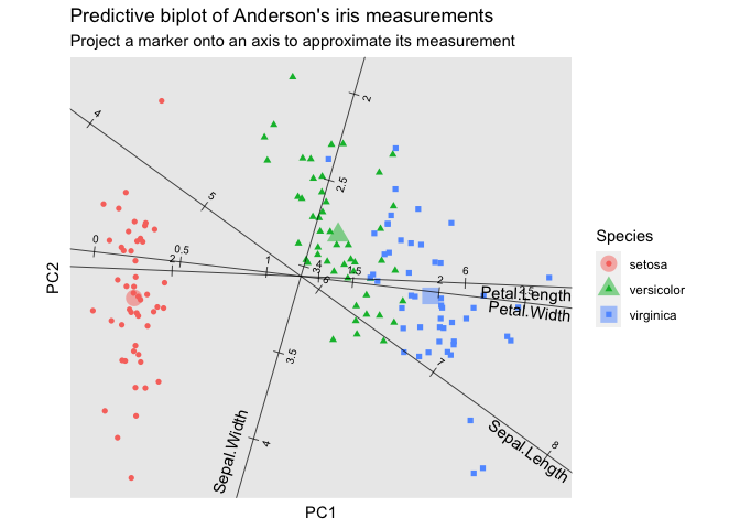
When variables are represented in standard coordinates, as typically in PCA, their rules can be rescaled to yield a predictive biplot.9 For legibility, the axes are limited to the data range and offset from the origin:
ggbiplot(iris_pca, axis.type = "predictive", axis.percents = FALSE) +
  theme_scaffold() +
  geom_rows_point(aes(color = Species, shape = Species)) +
  stat_rows_center(
    aes(color = Species, shape = Species),
    size = 5, alpha = .5, fun.data = mean_se
  ) +
  stat_cols_rule(aes(label = name, center = center, scale = scale)) +
  ggtitle("Predictive biplot of Anderson's iris measurements",
          "Project a marker onto an axis to approximate its measurement")
aggregate(iris[, 1:4], by = iris[, "Species", drop = FALSE], FUN = mean)
#>      Species Sepal.Length Sepal.Width Petal.Length Petal.Width
#> 1     setosa        5.006       3.428        1.462       0.246
#> 2 versicolor        5.936       2.770        4.260       1.326
#> 3  virginica        6.588       2.974        5.552       2.026
more methods
The auxiliary package ordr.extra provides recovery methods for several additional ordination models—and has room for several more!
acknowledgments
contribute
Any feedback on the package is very welcome! If you encounter confusion or errors, do create an issue, with a minimal reproducible example if feasible. If you have requests, suggestions, or your own implementations for new features, feel free to create an issue or submit a pull request. Methods for additional ordination classes (see the methods-*.r scripts in the R folder) are especially welcome, as are new plot layers. Please try to follow the contributing guidelines and respect the Code of Conduct.
inspirations
This package was originally inspired by the ggbiplot extension developed by Vincent Q. Vu, Richard J Telford, and Vilmantas Gegzna, among others. It probably first brought biplots into the Tidyverse framework. The motivation to unify a variety of ordination methods came from several books and articles by Michael Greenacre, in particular Biplots in Practice. Several answers at CrossValidated, in particular by amoeba and ttnphns, provided theoretical insights and informed design choices. Thomas Lin Pedersen’s tidygraph prequel to ggraph finally induced the shift from the downstream generation of scatterplots to the upstream handling and manipulating of models. Additional design elements and features have been informed by the monograph Biplots and the textbook Understanding Biplots by John C. Gower, David J. Hand, Sugnet Gardner–Lubbe, and Niël J. Le Roux, and by the volume Principal Components Analysis by I. T. Jolliffe.
exposition
This work was presented (slideshow PDF) at an invited panel on New Developments in Graphing Multivariate Data at the Joint Statistical Meetings, on 2022 August 8 in Washington DC. I’m grateful to Joyce Robbins for the invitation and for organizing such a fun first experience, to Naomi Robbins for chairing the event, and to my co-panelists Ursula Laa and Hengrui Luo for sharing and sparking such exciting ideas and conversations. An update was presented to the ggplot2 extenders, which elicited additional valuable feedback.
resources
Development of this package benefitted from the use of equipment and the support of colleagues at UConn Health and at UF Health.