Build a biplot visualization from ordination data wrapped as a tbl_ord object.
Usage
ggbiplot(
  ordination = NULL,
  mapping = aes(x = 1, y = 2),
  axis.type = "interpolative",
  xlim = NULL,
  ylim = NULL,
  expand = TRUE,
  clip = "on",
  axis.percents = TRUE,
  sec.axes = NULL,
  scale.factor = "inertia",
  scale_rows = NULL,
  scale_cols = NULL,
  ...
)

ord_aes(ordination, ...)
Arguments
- ordination
A tbl_ord.
- mapping
List of default aesthetic mappings to use for the biplot. The default assigns the first two coordinates to the aesthetics
xandy. Other assignments must be supplied in each layer added to the plot.- axis.type
Character, partially matched; whether to build an
"interpolative"(the default) or a"predictive"biplot. The latter requires thatxandyare mapped to shared coordinates, that no other shared coordinates are mapped to, and inertia is conferred entirely onto one matrix factor. NB: This option is only implemented for linear techniques (ED, SVD, & PCA).- xlim, ylim
Limits for the x and y axes.
- expand
If
TRUE, the default, adds a small expansion factor to the limits to ensure that data and axes don't overlap. IfFALSE, limits are taken exactly from the data orxlim/ylim.- clip
Should drawing be clipped to the extent of the plot panel? A setting of
"on"(the default) means yes, and a setting of"off"means no. In most cases, the default of"on"should not be changed, as settingclip = "off"can cause unexpected results. It allows drawing of data points anywhere on the plot, including in the plot margins. If limits are set viaxlimandylimand some data points fall outside those limits, then those data points may show up in places such as the axes, the legend, the plot title, or the plot margins.- axis.percents
Whether to concatenate default axis labels with inertia percentages.
- sec.axes
Matrix factor character to specify a secondary set of axes.
- scale.factor
Either a numeric value, used to scale the secondary axes against the primary axes, or the name of a harmonizing function (currently
"range"or"inertia"); ignored ifsec.axesis not specified.- scale_rows, scale_cols
Either the character name of a numeric variable in
get_*(ordination)or a numeric vector of lengthnrow(get_*(ordination)), used to scale the coordinates of the matrix factors.- ...
Additional arguments passed to
ggplot2::fortify(); seefortify.tbl_ord().
Value
A ggplot object.
Details
ggbiplot() produces a ggplot object from a tbl_ord
object ordination. The baseline object is the default unadorned
"ggplot"-class object p with the following differences from what
ggplot2::ggplot() returns:
p$mappingis augmented with.matrix = .matrix, which expects either.matrix = "rows"or.matrix = "cols"from the biplot.p$coordinatesis defaulted toggplot2::coord_equal()in order to faithfully render the geometry of an ordination. The optional parametersxlim,ylim,expand, andclipare passed tocoord_equal()and default to its ggplot2 defaults.When
xoryare mapped to coordinates ofordination, and ifaxis.percentsisTRUE,p$labels$xorp$labels$yare defaulted to the coordinate names concatenated with the percentages of inertia captured by the coordinates.pis assigned the class"ggbiplot"in addition to"ggplot". This serves no functional purpose currently.
Furthermore, the user may feed single integer values to the x and y
aesthetics, which will be interpreted as the corresponding coordinates in the
ordination. Currently only 2-dimensional biplots are supported, so both x
and y must take coordinate values.
ord_aes() is a convenience function that generates a full-rank set of
coordinate aesthetics ..coord1, ..coord2, etc. mapped to the shared
coordinates of the ordination object, along with any additional aesthetics
that are processed internally by ggplot2::aes().
The axis.type parameter controls whether the biplot is interpolative or
predictive, though predictive biplots are still experimental and limited to
linear methods like PCA. Gower & Hand (1996) and Gower, Gardner–Lubbe, & le
Roux (2011) thoroughly explain the construction and interpretation of
predictive biplots.
Biplot layers
ggbiplot() uses ggplot2::fortify() internally to produce a single data
frame with a .matrix column distinguishing the subjects ("rows") and
variables ("cols"). The stat layers stat_rows() and stat_cols() simply
filter the data frame to one of these two.
The geom layers geom_rows_*() and geom_cols_*() call the corresponding
stat in order to render plot elements for the corresponding factor matrix.
geom_dims_*() selects a default matrix based on common practice, e.g.
points for rows and arrows for columns.
References
Gower JC & Hand DJ (1996) Biplots. Chapman & Hall, ISBN: 0-412-71630-5.
Gower JC, Gardner–Lubbe S, & le Roux NJ (2011) Understanding Biplots. Wiley, ISBN: 978-0-470-01255-0. https://www.wiley.com/go/biplots
See also
ggplot2::ggplot2(), on which ggbiplot() is built
Examples
# compute PCA of Anderson iris measurements
iris[, -5] %>%
princomp(cor = TRUE) %>%
as_tbl_ord() %>%
confer_inertia(1) %>%
mutate_rows(species = iris$Species) %>%
mutate_cols(measure = gsub("\\.", " ", tolower(names(iris)[-5]))) %>%
print() -> iris_pca
#> # A tbl_ord of class 'princomp': (150 x 4) x (4 x 4)'
#> # 4 coordinates: Comp.1, Comp.2, ..., Comp.4
#> #
#> # Rows (principal): [ 150 x 4 | 1 ]
#> Comp.1 Comp.2 Comp.3 ... | species
#> | <fct>
#> 1 -2.26 0.480 0.128 | 1 setosa
#> 2 -2.08 -0.674 0.235 | 2 setosa
#> 3 -2.36 -0.342 -0.0442 ... | 3 setosa
#> 4 -2.30 -0.597 -0.0913 | 4 setosa
#> 5 -2.39 0.647 -0.0157 | 5 setosa
#> # ℹ 145 more rows | # ℹ 145 more rows
#>
#> #
#> # Columns (standard): [ 4 x 4 | 1 ]
#> Comp.1 Comp.2 Comp.3 ... | measure
#> | <chr>
#> 1 0.521 0.377 0.720 | 1 sepal length
#> 2 -0.269 0.923 -0.244 ... | 2 sepal width
#> 3 0.580 0.0245 -0.142 | 3 petal length
#> 4 0.565 0.0669 -0.634 | 4 petal width
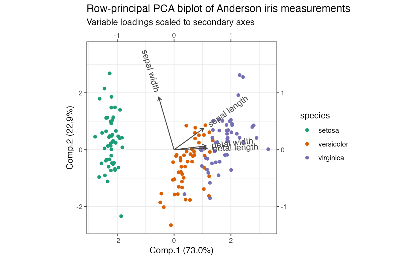
# row-principal biplot with range-harmonized secondary axis
iris_pca %>%
ggbiplot(aes(color = species), sec.axes = "cols", scale.factor = "range") +
theme_bw() +
scale_color_brewer(type = "qual", palette = 2) +
geom_rows_point() +
geom_cols_vector(aes(label = measure), color = "#444444") +
ggtitle(
"Row-principal PCA biplot of Anderson iris measurements",
"Variable loadings scaled to secondary axes"
) +
expand_limits(y = c(-1, 3.5))
 # row-principal biplot with manually rescaled secondary axis
iris_pca %>%
ggbiplot(aes(color = species), sec.axes = "cols", scale.factor = 2) +
theme_bw() +
scale_color_brewer(type = "qual", palette = 2) +
geom_rows_point() +
geom_cols_vector(aes(label = measure), color = "#444444") +
ggtitle(
"Row-principal PCA biplot of Anderson iris measurements",
"Variable loadings scaled to secondary axes"
) +
expand_limits(y = c(-1, 3.5))
# row-principal biplot with manually rescaled secondary axis
iris_pca %>%
ggbiplot(aes(color = species), sec.axes = "cols", scale.factor = 2) +
theme_bw() +
scale_color_brewer(type = "qual", palette = 2) +
geom_rows_point() +
geom_cols_vector(aes(label = measure), color = "#444444") +
ggtitle(
"Row-principal PCA biplot of Anderson iris measurements",
"Variable loadings scaled to secondary axes"
) +
expand_limits(y = c(-1, 3.5))
 # Performance measures can be regressed on the artificial coordinates of
# ordinated vehicle specs. Because the ordination of specs ignores performance,
# these coordinates will probably not be highly predictive. The gradient of each
# performance measure along the artificial axes is visualized by projecting the
# regression coefficients onto the ordination biplot.
# scaled principal components analysis of vehicle specs
mtcars_specs_pca <- ordinate(
mtcars, cols = c(cyl, disp, hp, drat, wt, vs, carb),
model = ~ princomp(., cor = TRUE)
)
# data frame of vehicle performance measures
mtcars %>%
subset(select = c(mpg, qsec)) %>%
as.matrix() %>%
print() -> mtcars_perf
#> mpg qsec
#> Mazda RX4 21.0 16.46
#> Mazda RX4 Wag 21.0 17.02
#> Datsun 710 22.8 18.61
#> Hornet 4 Drive 21.4 19.44
#> Hornet Sportabout 18.7 17.02
#> Valiant 18.1 20.22
#> Duster 360 14.3 15.84
#> Merc 240D 24.4 20.00
#> Merc 230 22.8 22.90
#> Merc 280 19.2 18.30
#> Merc 280C 17.8 18.90
#> Merc 450SE 16.4 17.40
#> Merc 450SL 17.3 17.60
#> Merc 450SLC 15.2 18.00
#> Cadillac Fleetwood 10.4 17.98
#> Lincoln Continental 10.4 17.82
#> Chrysler Imperial 14.7 17.42
#> Fiat 128 32.4 19.47
#> Honda Civic 30.4 18.52
#> Toyota Corolla 33.9 19.90
#> Toyota Corona 21.5 20.01
#> Dodge Challenger 15.5 16.87
#> AMC Javelin 15.2 17.30
#> Camaro Z28 13.3 15.41
#> Pontiac Firebird 19.2 17.05
#> Fiat X1-9 27.3 18.90
#> Porsche 914-2 26.0 16.70
#> Lotus Europa 30.4 16.90
#> Ford Pantera L 15.8 14.50
#> Ferrari Dino 19.7 15.50
#> Maserati Bora 15.0 14.60
#> Volvo 142E 21.4 18.60
# regress performance measures on principal components
lm(mtcars_perf ~ get_rows(mtcars_specs_pca)) %>%
as_tbl_ord() %>%
augment_ord() %>%
print() -> mtcars_pca_lm
#> # A tbl_ord of class 'mlm': (32 x 8) x (2 x 8)'
#> # 8 coordinates: (Intercept), Comp.1, ..., Comp.7
#> #
#> # Rows: [ 32 x 8 | 1 ]
#> `(Intercept)` Comp.1 Comp.2 ... | name
#> | <chr>
#> 1 1 -0.398 -1.12 | 1 Mazda RX4
#> 2 1 -0.294 -1.06 | 2 Mazda RX4 Wag
#> 3 1 -2.54 0.465 ... | 3 Datsun 710
#> 4 1 -0.601 1.75 | 4 Hornet 4 Drive
#> 5 1 1.61 0.837 | 5 Hornet Sportabout
#> # ℹ 27 more rows | # ℹ 27 more rows
#>
#> #
#> # Columns: [ 2 x 8 | 1 ]
#> `(Intercept)` Comp.1 Comp.2 ... | name
#> | <chr>
#> 1 20.1 -2.41 -0.415 ... | 1 mpg
#> 2 17.8 -0.459 0.929 | 2 qsec
# regression biplot
ggbiplot(mtcars_specs_pca, aes(label = name),
sec.axes = "rows", scale.factor = .5) +
theme_minimal() +
geom_rows_text(size = 3) +
geom_cols_vector(data = mtcars_pca_lm) +
expand_limits(x = c(-2.5, 2))
# Performance measures can be regressed on the artificial coordinates of
# ordinated vehicle specs. Because the ordination of specs ignores performance,
# these coordinates will probably not be highly predictive. The gradient of each
# performance measure along the artificial axes is visualized by projecting the
# regression coefficients onto the ordination biplot.
# scaled principal components analysis of vehicle specs
mtcars_specs_pca <- ordinate(
mtcars, cols = c(cyl, disp, hp, drat, wt, vs, carb),
model = ~ princomp(., cor = TRUE)
)
# data frame of vehicle performance measures
mtcars %>%
subset(select = c(mpg, qsec)) %>%
as.matrix() %>%
print() -> mtcars_perf
#> mpg qsec
#> Mazda RX4 21.0 16.46
#> Mazda RX4 Wag 21.0 17.02
#> Datsun 710 22.8 18.61
#> Hornet 4 Drive 21.4 19.44
#> Hornet Sportabout 18.7 17.02
#> Valiant 18.1 20.22
#> Duster 360 14.3 15.84
#> Merc 240D 24.4 20.00
#> Merc 230 22.8 22.90
#> Merc 280 19.2 18.30
#> Merc 280C 17.8 18.90
#> Merc 450SE 16.4 17.40
#> Merc 450SL 17.3 17.60
#> Merc 450SLC 15.2 18.00
#> Cadillac Fleetwood 10.4 17.98
#> Lincoln Continental 10.4 17.82
#> Chrysler Imperial 14.7 17.42
#> Fiat 128 32.4 19.47
#> Honda Civic 30.4 18.52
#> Toyota Corolla 33.9 19.90
#> Toyota Corona 21.5 20.01
#> Dodge Challenger 15.5 16.87
#> AMC Javelin 15.2 17.30
#> Camaro Z28 13.3 15.41
#> Pontiac Firebird 19.2 17.05
#> Fiat X1-9 27.3 18.90
#> Porsche 914-2 26.0 16.70
#> Lotus Europa 30.4 16.90
#> Ford Pantera L 15.8 14.50
#> Ferrari Dino 19.7 15.50
#> Maserati Bora 15.0 14.60
#> Volvo 142E 21.4 18.60
# regress performance measures on principal components
lm(mtcars_perf ~ get_rows(mtcars_specs_pca)) %>%
as_tbl_ord() %>%
augment_ord() %>%
print() -> mtcars_pca_lm
#> # A tbl_ord of class 'mlm': (32 x 8) x (2 x 8)'
#> # 8 coordinates: (Intercept), Comp.1, ..., Comp.7
#> #
#> # Rows: [ 32 x 8 | 1 ]
#> `(Intercept)` Comp.1 Comp.2 ... | name
#> | <chr>
#> 1 1 -0.398 -1.12 | 1 Mazda RX4
#> 2 1 -0.294 -1.06 | 2 Mazda RX4 Wag
#> 3 1 -2.54 0.465 ... | 3 Datsun 710
#> 4 1 -0.601 1.75 | 4 Hornet 4 Drive
#> 5 1 1.61 0.837 | 5 Hornet Sportabout
#> # ℹ 27 more rows | # ℹ 27 more rows
#>
#> #
#> # Columns: [ 2 x 8 | 1 ]
#> `(Intercept)` Comp.1 Comp.2 ... | name
#> | <chr>
#> 1 20.1 -2.41 -0.415 ... | 1 mpg
#> 2 17.8 -0.459 0.929 | 2 qsec
# regression biplot
ggbiplot(mtcars_specs_pca, aes(label = name),
sec.axes = "rows", scale.factor = .5) +
theme_minimal() +
geom_rows_text(size = 3) +
geom_cols_vector(data = mtcars_pca_lm) +
expand_limits(x = c(-2.5, 2))
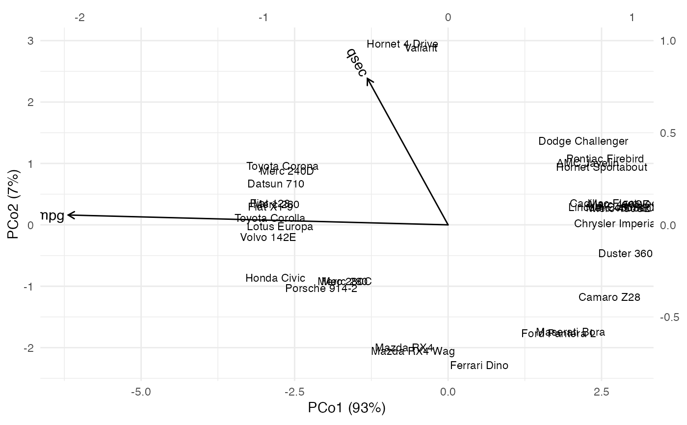 # multidimensional scaling based on a scaled cosine distance of vehicle specs
cosine_dist <- function(x) {
x <- as.matrix(x)
num <- x %*% t(x)
denom_rt <- as.matrix(rowSums(x^2))
denom <- sqrt(denom_rt %*% t(denom_rt))
as.dist(1 - num / denom)
}
mtcars %>%
subset(select = c(cyl, disp, hp, drat, wt, vs, carb)) %>%
scale() %>%
cosine_dist() %>%
cmdscale() %>%
as.data.frame() ->
mtcars_specs_cmds
# names must be consistent with `cmdscale_ord()` below
names(mtcars_specs_cmds) <- c("PCo1", "PCo2")
# regress performance measures on principal coordinates
lm(mtcars_perf ~ as.matrix(mtcars_specs_cmds)) %>%
as_tbl_ord() %>%
augment_ord() %>%
print() -> mtcars_cmds_lm
#> # A tbl_ord of class 'mlm': (32 x 3) x (2 x 3)'
#> # 3 coordinates: (Intercept), PCo1, PCo2
#> #
#> # Rows: [ 32 x 3 | 1 ]
#> `(Intercept)` PCo1 PCo2 | name
#> | <chr>
#> 1 1 -0.238 -0.666 | 1 Mazda RX4
#> 2 1 -0.190 -0.685 | 2 Mazda RX4 Wag
#> 3 1 -0.934 0.224 | 3 Datsun 710
#> 4 1 -0.247 0.984 | 4 Hornet 4 Drive
#> 5 1 0.834 0.316 | 5 Hornet Sportabout
#> # ℹ 27 more rows | # ℹ 27 more rows
#>
#> #
#> # Columns: [ 2 x 3 | 1 ]
#> `(Intercept)` PCo1 PCo2 | name
#> | <chr>
#> 1 20.1 -6.19 0.160 | 1 mpg
#> 2 17.8 -1.31 2.38 | 2 qsec
# multidimensional scaling using `cmdscale_ord()`
mtcars %>%
subset(select = c(cyl, disp, hp, drat, wt, vs, carb)) %>%
scale() %>%
cosine_dist() %>%
cmdscale_ord() %>%
as_tbl_ord() %>%
augment_ord() %>%
print() -> mtcars_specs_cmds_ord
#> # A tbl_ord of class 'cmds_ord': (32 x 2) x (32 x 2)'
#> # 2 coordinates: PCo1 and PCo2
#> #
#> # Rows (symmetric): [ 32 x 2 | 1 ]
#> PCo1 PCo2 | name
#> | <chr>
#> 1 -0.238 -0.666 | 1 Mazda RX4
#> 2 -0.190 -0.685 | 2 Mazda RX4 Wag
#> 3 -0.934 0.224 | 3 Datsun 710
#> 4 -0.247 0.984 | 4 Hornet 4 Drive
#> 5 0.834 0.316 | 5 Hornet Sportabout
#> # ℹ 27 more rows | # ℹ 27 more rows
#>
#> #
#> # Columns (symmetric): [ 32 x 2 | 1 ]
#> PCo1 PCo2 | name
#> | <chr>
#> 1 -0.238 -0.666 | 1 Mazda RX4
#> 2 -0.190 -0.685 | 2 Mazda RX4 Wag
#> 3 -0.934 0.224 | 3 Datsun 710
#> 4 -0.247 0.984 | 4 Hornet 4 Drive
#> 5 0.834 0.316 | 5 Hornet Sportabout
#> # ℹ 27 more rows | # ℹ 27 more rows
#>
# regression biplot
ggbiplot(mtcars_specs_cmds_ord, aes(label = name),
sec.axes = "rows", scale.factor = 3) +
theme_minimal() +
geom_rows_text(size = 3) +
geom_cols_vector(data = mtcars_cmds_lm) +
expand_limits(x = c(-2.25, 1.25), y = c(-2, 1.5))
# multidimensional scaling based on a scaled cosine distance of vehicle specs
cosine_dist <- function(x) {
x <- as.matrix(x)
num <- x %*% t(x)
denom_rt <- as.matrix(rowSums(x^2))
denom <- sqrt(denom_rt %*% t(denom_rt))
as.dist(1 - num / denom)
}
mtcars %>%
subset(select = c(cyl, disp, hp, drat, wt, vs, carb)) %>%
scale() %>%
cosine_dist() %>%
cmdscale() %>%
as.data.frame() ->
mtcars_specs_cmds
# names must be consistent with `cmdscale_ord()` below
names(mtcars_specs_cmds) <- c("PCo1", "PCo2")
# regress performance measures on principal coordinates
lm(mtcars_perf ~ as.matrix(mtcars_specs_cmds)) %>%
as_tbl_ord() %>%
augment_ord() %>%
print() -> mtcars_cmds_lm
#> # A tbl_ord of class 'mlm': (32 x 3) x (2 x 3)'
#> # 3 coordinates: (Intercept), PCo1, PCo2
#> #
#> # Rows: [ 32 x 3 | 1 ]
#> `(Intercept)` PCo1 PCo2 | name
#> | <chr>
#> 1 1 -0.238 -0.666 | 1 Mazda RX4
#> 2 1 -0.190 -0.685 | 2 Mazda RX4 Wag
#> 3 1 -0.934 0.224 | 3 Datsun 710
#> 4 1 -0.247 0.984 | 4 Hornet 4 Drive
#> 5 1 0.834 0.316 | 5 Hornet Sportabout
#> # ℹ 27 more rows | # ℹ 27 more rows
#>
#> #
#> # Columns: [ 2 x 3 | 1 ]
#> `(Intercept)` PCo1 PCo2 | name
#> | <chr>
#> 1 20.1 -6.19 0.160 | 1 mpg
#> 2 17.8 -1.31 2.38 | 2 qsec
# multidimensional scaling using `cmdscale_ord()`
mtcars %>%
subset(select = c(cyl, disp, hp, drat, wt, vs, carb)) %>%
scale() %>%
cosine_dist() %>%
cmdscale_ord() %>%
as_tbl_ord() %>%
augment_ord() %>%
print() -> mtcars_specs_cmds_ord
#> # A tbl_ord of class 'cmds_ord': (32 x 2) x (32 x 2)'
#> # 2 coordinates: PCo1 and PCo2
#> #
#> # Rows (symmetric): [ 32 x 2 | 1 ]
#> PCo1 PCo2 | name
#> | <chr>
#> 1 -0.238 -0.666 | 1 Mazda RX4
#> 2 -0.190 -0.685 | 2 Mazda RX4 Wag
#> 3 -0.934 0.224 | 3 Datsun 710
#> 4 -0.247 0.984 | 4 Hornet 4 Drive
#> 5 0.834 0.316 | 5 Hornet Sportabout
#> # ℹ 27 more rows | # ℹ 27 more rows
#>
#> #
#> # Columns (symmetric): [ 32 x 2 | 1 ]
#> PCo1 PCo2 | name
#> | <chr>
#> 1 -0.238 -0.666 | 1 Mazda RX4
#> 2 -0.190 -0.685 | 2 Mazda RX4 Wag
#> 3 -0.934 0.224 | 3 Datsun 710
#> 4 -0.247 0.984 | 4 Hornet 4 Drive
#> 5 0.834 0.316 | 5 Hornet Sportabout
#> # ℹ 27 more rows | # ℹ 27 more rows
#>
# regression biplot
ggbiplot(mtcars_specs_cmds_ord, aes(label = name),
sec.axes = "rows", scale.factor = 3) +
theme_minimal() +
geom_rows_text(size = 3) +
geom_cols_vector(data = mtcars_cmds_lm) +
expand_limits(x = c(-2.25, 1.25), y = c(-2, 1.5))
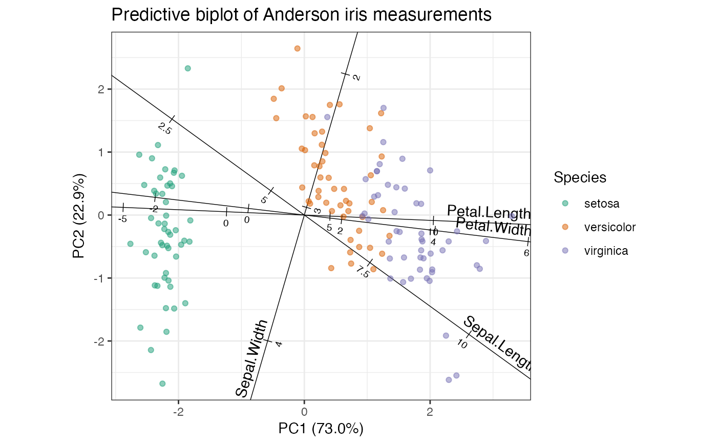
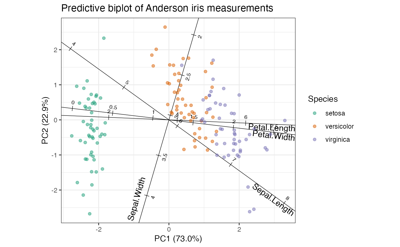 # PCA of iris data
iris_pca <- ordinate(iris, cols = 1:4, prcomp, scale = TRUE)
# row-principal predictive biplot
iris_pca %>%
ggbiplot(axis.type = "predictive") +
theme_bw() +
scale_color_brewer(type = "qual", palette = 2) +
geom_cols_axis(aes(label = name, center = center, scale = scale)) +
geom_rows_point(aes(color = Species), alpha = .5) +
ggtitle("Predictive biplot of Anderson iris measurements")
# PCA of iris data
iris_pca <- ordinate(iris, cols = 1:4, prcomp, scale = TRUE)
# row-principal predictive biplot
iris_pca %>%
ggbiplot(axis.type = "predictive") +
theme_bw() +
scale_color_brewer(type = "qual", palette = 2) +
geom_cols_axis(aes(label = name, center = center, scale = scale)) +
geom_rows_point(aes(color = Species), alpha = .5) +
ggtitle("Predictive biplot of Anderson iris measurements")
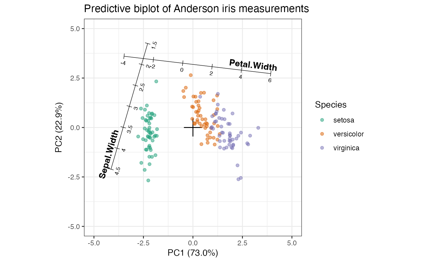
 # with two calibrated axes
iris_pca %>%
ggbiplot(axis.type = "predictive") +
theme_bw() +
scale_color_brewer(type = "qual", palette = 2) +
geom_origin() +
stat_cols_rule(
subset = c(2, 4), fontface = "bold", text.fontface = "plain",
aes(label = name, center = center, scale = scale)
) +
geom_rows_point(aes(color = Species), alpha = .5) +
expand_limits(x = c(-5, 5), y = c(-5, 5)) +
ggtitle("Predictive biplot of Anderson iris measurements")
# with two calibrated axes
iris_pca %>%
ggbiplot(axis.type = "predictive") +
theme_bw() +
scale_color_brewer(type = "qual", palette = 2) +
geom_origin() +
stat_cols_rule(
subset = c(2, 4), fontface = "bold", text.fontface = "plain",
aes(label = name, center = center, scale = scale)
) +
geom_rows_point(aes(color = Species), alpha = .5) +
expand_limits(x = c(-5, 5), y = c(-5, 5)) +
ggtitle("Predictive biplot of Anderson iris measurements")