Functionality for multiple correspondence analysis ('mca') objects
Source:R/methods-mass-mca.r
methods-mca.RdThese methods extract data from, and attribute new data to,
objects of class "mca" from the MASS package.
Usage
# S3 method for class 'mca'
as_tbl_ord(x)

# S3 method for class 'mca'
recover_rows(x)

# S3 method for class 'mca'
recover_cols(x)

# S3 method for class 'mca'
recover_inertia(x)

# S3 method for class 'mca'
recover_conference(x)

# S3 method for class 'mca'
recover_coord(x)

# S3 method for class 'mca'
recover_supp_rows(x)

# S3 method for class 'mca'
recover_aug_rows(x)

# S3 method for class 'mca'
recover_aug_cols(x)

# S3 method for class 'mca'
recover_aug_coord(x)Value
The recovery generics recover_*() return core model components, distribution of inertia,
supplementary elements, and intrinsic metadata; but they require methods for each model class to
tell them what these components are.
The generic as_tbl_ord() returns its input wrapped in the 'tbl_ord'
class. Its methods determine what model classes it is allowed to wrap. It
then provides 'tbl_ord' methods with access to the recoverers and hence to
the model components.
Details
Multiple correspondence analysis (MCA) relies on a singular value
decomposition of the indicator matrix \(X\) of a table of several
categorical variables, scaled by its column totals. MASS::mca() returns the
SVD factors \(UD\) and \(V\) as the row weights $fs, on which the
inertia is conferred, and the column coordinates $cs. The row coordinates
$rs are obtained as \(XV\) and accessible as supplementary elements.
See also
Other methods for singular value decomposition-based techniques:
methods-cancor,
methods-correspondence,
methods-lda,
methods-lra,
methods-prcomp,
methods-svd
Other models from the MASS package:
methods-correspondence,
methods-lda
Examples
# table of admissions and rejections from UC Berkeley
class(UCBAdmissions)
#> [1] "table"
ucb_admissions <- as.data.frame(UCBAdmissions)
ucb_admissions <-
  ucb_admissions[rep(seq(nrow(ucb_admissions)), ucb_admissions$Freq), -4L]
head(ucb_admissions)
#>        Admit Gender Dept
#> 1   Admitted   Male    A
#> 1.1 Admitted   Male    A
#> 1.2 Admitted   Male    A
#> 1.3 Admitted   Male    A
#> 1.4 Admitted   Male    A
#> 1.5 Admitted   Male    A
# perform multiple correspondence analysis
ucb_admissions %>%
  MASS::mca() %>%
  as_tbl_ord() %>%
  # augment profiles with names, masses, distances, and inertias
  augment_ord() %>%
  print() -> admissions_mca
#> # A tbl_ord of class 'mca': (9052 x 2) x (10 x 2)'
#> # 2 coordinates: Dim1 and Dim2
#> #
#> # Rows (principal): [ 9052 x 2 | 2 ]
#>       Dim1     Dim2 |   name  .element
#>                     |   <chr> <chr>
#> 1 -0.01000 -0.00261 | 1 1     active
#> 2 -0.01000 -0.00261 | 2 1.1   active
#> 3 -0.01000 -0.00261 | 3 1.2   active
#> 4 -0.01000 -0.00261 | 4 1.3   active
#> 5 -0.01000 -0.00261 | 5 1.4   active
#> # ℹ 9,047 more rows | # ℹ 9,047 more rows
#>
#> #
#> # Columns (standard): [ 10 x 2 | 4 ]
#>        Dim1      Dim2 |    name        factor level .element
#>                       |    <chr>       <chr>  <chr> <chr>
#>  1 -0.00533 -0.00483  |  1 Admit.Admi… Admit  Admi… active
#>  2  0.00338  0.00306  |  2 Admit.Reje… Admit  Reje… active
#>  3 -0.00397  0.00266  |  3 Gender.Male Gender Male  active
#>  4  0.00582 -0.00390  |  4 Gender.Fem… Gender Fema… active
#>  5 -0.00748 -0.000829 |  5 Dept.A      Dept   A     active
#>  6 -0.00838  0.00295  |  6 Dept.B      Dept   B     active
#>  7  0.00395 -0.00851  |  7 Dept.C      Dept   C     active
#>  8  0.00160 -0.000439 |  8 Dept.D      Dept   D     active
#>  9  0.00561 -0.00450  |  9 Dept.E      Dept   E     active
#> 10  0.00519  0.0138   | 10 Dept.F      Dept   F     active

# recover row and column coordinates and row weights
head(get_rows(admissions_mca, elements = "score"))
#>             Dim1         Dim2
#> 1   -0.005592325 -0.001001186
#> 1.1 -0.005592325 -0.001001186
#> 1.2 -0.005592325 -0.001001186
#> 1.3 -0.005592325 -0.001001186
#> 1.4 -0.005592325 -0.001001186
#> 1.5 -0.005592325 -0.001001186
get_cols(admissions_mca)
#>                        Dim1          Dim2
#> Admit.Admitted -0.005329295 -0.0048307823
#> Admit.Rejected  0.003375284  0.0030595536
#> Gender.Male    -0.003971450  0.0026563610
#> Gender.Female   0.005824072 -0.0038955136
#> Dept.A         -0.007476230 -0.0008291371
#> Dept.B         -0.008381159  0.0029516575
#> Dept.C          0.003949742 -0.0085082718
#> Dept.D          0.001600698 -0.0004388113
#> Dept.E          0.005610973 -0.0045007472
#> Dept.F          0.005193103  0.0137723160
head(get_rows(admissions_mca))
#>             Dim1         Dim2
#> 1   -0.009997779 -0.002609712
#> 1.1 -0.009997779 -0.002609712
#> 1.2 -0.009997779 -0.002609712
#> 1.3 -0.009997779 -0.002609712
#> 1.4 -0.009997779 -0.002609712
#> 1.5 -0.009997779 -0.002609712

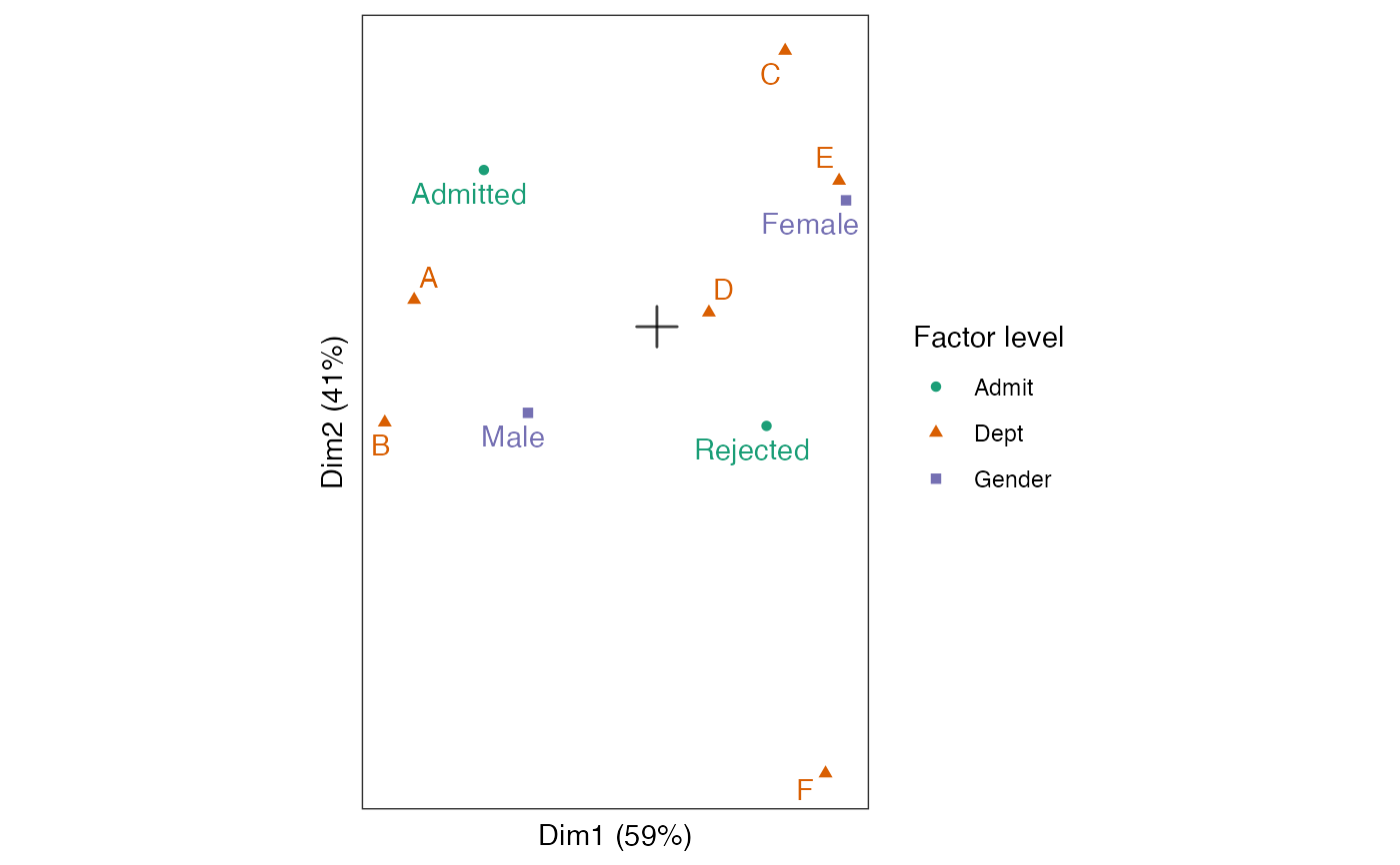
# column-standard biplot of factor levels
admissions_mca %>%
  ggbiplot() +
  theme_bw() + theme_biplot() +
  geom_origin() +
  #geom_rows_point(stat = "unique") +
  geom_cols_point(aes(color = factor, shape = factor)) +
  geom_cols_text_repel(aes(label = level, color = factor),
                       show.legend = FALSE) +
  scale_color_brewer(palette = "Dark2") +
  scale_size_area(guide = "none") +
  labs(color = "Factor level", shape = "Factor level")
