These statistical transformations (stats) adapt
conventional ggplot2 stats to one or the other matrix factor
of a tbl_ord, in lieu of stat_rows() or stat_cols(). They
accept the same parameters as their corresponding conventional
stats.
Usage
stat_rows_density_2d(
  mapping = NULL,
  data = NULL,
  geom = "density_2d",
  position = "identity",
  ...,
  contour = TRUE,
  contour_var = "density",
  n = 100,
  h = NULL,
  adjust = c(1, 1),
  na.rm = FALSE,
  show.legend = NA,
  inherit.aes = TRUE
)

stat_cols_density_2d(
  mapping = NULL,
  data = NULL,
  geom = "density_2d",
  position = "identity",
  ...,
  contour = TRUE,
  contour_var = "density",
  n = 100,
  h = NULL,
  adjust = c(1, 1),
  na.rm = FALSE,
  show.legend = NA,
  inherit.aes = TRUE
)

stat_rows_density_2d_filled(
  mapping = NULL,
  data = NULL,
  geom = "density_2d_filled",
  position = "identity",
  ...,
  contour = TRUE,
  contour_var = "density",
  n = 100,
  h = NULL,
  adjust = c(1, 1),
  na.rm = FALSE,
  show.legend = NA,
  inherit.aes = TRUE
)

stat_cols_density_2d_filled(
  mapping = NULL,
  data = NULL,
  geom = "density_2d_filled",
  position = "identity",
  ...,
  contour = TRUE,
  contour_var = "density",
  n = 100,
  h = NULL,
  adjust = c(1, 1),
  na.rm = FALSE,
  show.legend = NA,
  inherit.aes = TRUE
)

stat_rows_ellipse(
  mapping = NULL,
  data = NULL,
  geom = "path",
  position = "identity",
  ...,
  type = "t",
  level = 0.95,
  segments = 51,
  na.rm = FALSE,
  show.legend = NA,
  inherit.aes = TRUE
)

stat_cols_ellipse(
  mapping = NULL,
  data = NULL,
  geom = "path",
  position = "identity",
  ...,
  type = "t",
  level = 0.95,
  segments = 51,
  na.rm = FALSE,
  show.legend = NA,
  inherit.aes = TRUE
)

stat_rows_center(
  mapping = NULL,
  data = NULL,
  geom = "point",
  position = "identity",
  show.legend = NA,
  inherit.aes = TRUE,
  ...,
  fun.data = NULL,
  fun = NULL,
  fun.center = NULL,
  fun.min = NULL,
  fun.max = NULL,
  fun.ord = NULL,
  fun.args = list()
)

stat_cols_center(
  mapping = NULL,
  data = NULL,
  geom = "point",
  position = "identity",
  show.legend = NA,
  inherit.aes = TRUE,
  ...,
  fun.data = NULL,
  fun = NULL,
  fun.center = NULL,
  fun.min = NULL,
  fun.max = NULL,
  fun.ord = NULL,
  fun.args = list()
)

stat_rows_star(
  mapping = NULL,
  data = NULL,
  geom = "segment",
  position = "identity",
  show.legend = NA,
  inherit.aes = TRUE,
  ...,
  fun.data = NULL,
  fun = NULL,
  fun.center = NULL,
  fun.ord = NULL,
  fun.args = list()
)

stat_cols_star(
  mapping = NULL,
  data = NULL,
  geom = "segment",
  position = "identity",
  show.legend = NA,
  inherit.aes = TRUE,
  ...,
  fun.data = NULL,
  fun = NULL,
  fun.center = NULL,
  fun.ord = NULL,
  fun.args = list()
)

stat_rows_chull(
  mapping = NULL,
  data = NULL,
  geom = "polygon",
  position = "identity",
  show.legend = NA,
  inherit.aes = TRUE,
  ...
)

stat_cols_chull(
  mapping = NULL,
  data = NULL,
  geom = "polygon",
  position = "identity",
  show.legend = NA,
  inherit.aes = TRUE,
  ...
)

stat_rows_peel(
  mapping = NULL,
  data = NULL,
  geom = "polygon",
  position = "identity",
  num = NULL,
  by = 1L,
  breaks = c(0.5),
  cut = c("above", "below"),
  show.legend = NA,
  inherit.aes = TRUE,
  ...
)

stat_cols_peel(
  mapping = NULL,
  data = NULL,
  geom = "polygon",
  position = "identity",
  num = NULL,
  by = 1L,
  breaks = c(0.5),
  cut = c("above", "below"),
  show.legend = NA,
  inherit.aes = TRUE,
  ...
)

stat_rows_cone(
  mapping = NULL,
  data = NULL,
  geom = "path",
  position = "identity",
  origin = FALSE,
  show.legend = NA,
  inherit.aes = TRUE,
  ...
)

stat_cols_cone(
  mapping = NULL,
  data = NULL,
  geom = "path",
  position = "identity",
  origin = FALSE,
  show.legend = NA,
  inherit.aes = TRUE,
  ...
)

stat_rows_depth(
  mapping = NULL,
  data = NULL,
  geom = "contour",
  position = "identity",
  contour = TRUE,
  contour_var = "depth",
  notion = "zonoid",
  notion_params = list(),
  n = 100L,
  show.legend = NA,
  inherit.aes = TRUE,
  ...
)

stat_cols_depth(
  mapping = NULL,
  data = NULL,
  geom = "contour",
  position = "identity",
  contour = TRUE,
  contour_var = "depth",
  notion = "zonoid",
  notion_params = list(),
  n = 100L,
  show.legend = NA,
  inherit.aes = TRUE,
  ...
)

stat_rows_depth_filled(
  mapping = NULL,
  data = NULL,
  geom = "contour_filled",
  position = "identity",
  contour = TRUE,
  contour_var = "depth",
  notion = "zonoid",
  notion_params = list(),
  n = 100L,
  show.legend = NA,
  inherit.aes = TRUE,
  ...
)

stat_cols_depth_filled(
  mapping = NULL,
  data = NULL,
  geom = "contour_filled",
  position = "identity",
  contour = TRUE,
  contour_var = "depth",
  notion = "zonoid",
  notion_params = list(),
  n = 100L,
  show.legend = NA,
  inherit.aes = TRUE,
  ...
)

stat_rows_scale(
  mapping = NULL,
  data = NULL,
  geom = "point",
  position = "identity",
  show.legend = NA,
  inherit.aes = TRUE,
  ...,
  mult = 1
)

stat_cols_scale(
  mapping = NULL,
  data = NULL,
  geom = "point",
  position = "identity",
  show.legend = NA,
  inherit.aes = TRUE,
  ...,
  mult = 1
)

stat_rows_spantree(
  mapping = NULL,
  data = NULL,
  geom = "segment",
  position = "identity",
  engine = "mlpack",
  method = "euclidean",
  show.legend = NA,
  inherit.aes = TRUE,
  ...
)

stat_cols_spantree(
  mapping = NULL,
  data = NULL,
  geom = "segment",
  position = "identity",
  engine = "mlpack",
  method = "euclidean",
  show.legend = NA,
  inherit.aes = TRUE,
  ...
)

stat_rows_bagplot(
  mapping = NULL,
  data = NULL,
  geom = "bagplot",
  position = "identity",
  fraction = 0.5,
  coef = 3,
  median = TRUE,
  fence = TRUE,
  outliers = TRUE,
  show.legend = NA,
  inherit.aes = TRUE,
  ...
)

stat_cols_bagplot(
  mapping = NULL,
  data = NULL,
  geom = "bagplot",
  position = "identity",
  fraction = 0.5,
  coef = 3,
  median = TRUE,
  fence = TRUE,
  outliers = TRUE,
  show.legend = NA,
  inherit.aes = TRUE,
  ...
)

stat_rows_rule(
  mapping = NULL,
  data = NULL,
  geom = "rule",
  position = "identity",
  fun.lower = "minpp",
  fun.upper = "maxpp",
  fun.offset = "minabspp",
  fun.args = list(),
  referent = NULL,
  show.legend = NA,
  inherit.aes = TRUE,
  ref_subset = NULL,
  ref_elements = "active",
  ...
)

stat_cols_rule(
  mapping = NULL,
  data = NULL,
  geom = "rule",
  position = "identity",
  fun.lower = "minpp",
  fun.upper = "maxpp",
  fun.offset = "minabspp",
  fun.args = list(),
  referent = NULL,
  show.legend = NA,
  inherit.aes = TRUE,
  ref_subset = NULL,
  ref_elements = "active",
  ...
)

stat_rows_projection(
  mapping = NULL,
  data = NULL,
  geom = "segment",
  position = "identity",
  referent = NULL,
  ref_subset = NULL,
  ref_elements = "active",
  ...,
  show.legend = NA,
  inherit.aes = TRUE
)

stat_cols_projection(
  mapping = NULL,
  data = NULL,
  geom = "segment",
  position = "identity",
  referent = NULL,
  ref_subset = NULL,
  ref_elements = "active",
  ...,
  show.legend = NA,
  inherit.aes = TRUE
)
Arguments
- mapping
Set of aesthetic mappings created by
aes(). If specified andinherit.aes = TRUE(the default), it is combined with the default mapping at the top level of the plot. You must supplymappingif there is no plot mapping.- data
The data to be displayed in this layer. There are three options:
If
NULL, the default, the data is inherited from the plot data as specified in the call toggplot().A
data.frame, or other object, will override the plot data. All objects will be fortified to produce a data frame. Seefortify()for which variables will be created.A
functionwill be called with a single argument, the plot data. The return value must be adata.frame, and will be used as the layer data. Afunctioncan be created from aformula(e.g.~ head(.x, 10)).- geom
The geometric object to use to display the data for this layer. When using a
stat_*()function to construct a layer, thegeomargument can be used to override the default coupling between stats and geoms. Thegeomargument accepts the following:A
Geomggproto subclass, for exampleGeomPoint.A string naming the geom. To give the geom as a string, strip the function name of the
geom_prefix. For example, to usegeom_point(), give the geom as"point".For more information and other ways to specify the geom, see the layer geom documentation.
- position
A position adjustment to use on the data for this layer. This can be used in various ways, including to prevent overplotting and improving the display. The
positionargument accepts the following:The result of calling a position function, such as
position_jitter(). This method allows for passing extra arguments to the position.A string naming the position adjustment. To give the position as a string, strip the function name of the
position_prefix. For example, to useposition_jitter(), give the position as"jitter".For more information and other ways to specify the position, see the layer position documentation.
- ...
Additional arguments passed to
ggplot2::layer().- contour
If
TRUE, contour the results of the 2d density estimation.- contour_var
Character string identifying the variable to contour by. Can be one of
"density","ndensity", or"count". See the section on computed variables for details.- n
Number of grid points in each direction.
- h
Bandwidth (vector of length two). If
NULL, estimated usingMASS::bandwidth.nrd().- adjust
A multiplicative bandwidth adjustment to be used if 'h' is 'NULL'. This makes it possible to adjust the bandwidth while still using the a bandwidth estimator. For example,
adjust = 1/2means use half of the default bandwidth.- na.rm
If
FALSE, the default, missing values are removed with a warning. IfTRUE, missing values are silently removed.- show.legend
logical. Should this layer be included in the legends?
NA, the default, includes if any aesthetics are mapped.FALSEnever includes, andTRUEalways includes. It can also be a named logical vector to finely select the aesthetics to display.- inherit.aes
If
FALSE, overrides the default aesthetics, rather than combining with them. This is most useful for helper functions that define both data and aesthetics and shouldn't inherit behaviour from the default plot specification, e.g.borders().- type
The type of ellipse. The default
"t"assumes a multivariate t-distribution, and"norm"assumes a multivariate normal distribution."euclid"draws a circle with the radius equal tolevel, representing the euclidean distance from the center. This ellipse probably won't appear circular unlesscoord_fixed()is applied.- level
The level at which to draw an ellipse, or, if
type="euclid", the radius of the circle to be drawn.- segments
The number of segments to be used in drawing the ellipse.
- fun.data
A function that is given the complete data and should return a data frame with variables
ymin,y, andymax.- fun.center
Deprecated alias to
fun.- fun.min, fun, fun.max
Alternatively, supply three individual functions that are each passed a vector of values and should return a single number.
- fun.ord
Alternatively to the
ggplot2::stat_summary_bin()parameters, supply a summary function that takes a matrix as input and returns a named column summary vector. Overridden byfun.dataandfun, cannot be used together withfun.minandfun.max.- fun.args
Optional additional arguments passed on to the functions.
- num
A positive integer; the number of hulls to peel. Pass
Inffor all hulls.- by
A positive integer; with what frequency to include consecutive hulls, pairs with
num.- breaks
A numeric vector of fractions (between
0and1) of the data to contain in each hull; overridden bynum.- cut
Character; one of
"above"and"below", indicating whether each hull should contain at least or at mostbreaksof the data, respectively.- origin
Logical; whether to include the origin with the transformed data. Defaults to
FALSE.- notion
Character; the name of the depth function (passed to
ddalpha::depth.()).- notion_params
List of additional parameters passed via
...toddalpha::depth.().- mult
Numeric value used to scale the coordinates.
- engine
A single character string specifying the package implementation to use;
"mlpack","vegan", or"ade4".- method
Passed to
stats::dist()ifengineis"vegan"or"ade4", ignored if"mlpack".- fraction
Fraction of the data to include in the bag.
- coef
Scale factor of the fence relative to the bag.
- median, fence, outliers
Logical indicators whether to include median, fence, and outliers in the composite output.
- fun.lower, fun.upper, fun.offset
Functions used to determine the limits of the rules and the translations of the axes from the projections of
referentonto the axes and onto their normal vectors.- referent
The reference data set; see Details.
- ref_elements, ref_subset
Analogues of
elementsandsubsetapplied toreferent.
Value
A ggproto layer.
Ordination aesthetics
This statistical transformation is compatible with the convenience function
ord_aes().
Some transformations (e.g. stat_center()) commute with projection to the
lower (1 or 2)-dimensional biplot space. If they detect aesthetics of the
form ..coord[0-9]+, then ..coord1 and ..coord2 are converted to x and
y while any remaining are ignored.
Other transformations (e.g. stat_spantree()) yield different results in a
lower-dimensional biplot when they are computed before versus after
projection. If the stat layer detects these aesthetics, then the
transformation is performed before projection, and the results in the first
two dimensions are returned as x and y.
A small number of transformations (stat_rule()) are incompatible with
ordination aesthetics but will accept ord_aes() without warning.
See also
Other biplot layers:
biplot-geoms,
stat_rows()
Examples
iris_pca <- ordinate(iris, prcomp, cols = seq(4), scale. = TRUE)
# NB: Non-standard aesthetics are handled as in version > 3.5.1; see:
# https://github.com/tidyverse/ggplot2/issues/6191
# This prevents `scale_color_discrete(aesthetics = ...)` from synching them.
ggbiplot(iris_pca) +
stat_rows_bagplot(
aes(fill = Species),
median_gp = list(color = sync()),
fence_gp = list(linewidth = 0.25),
outlier_gp = list(shape = "asterisk")
) +
scale_color_discrete(name = "Species", aesthetics = c("color", "fill")) +
geom_cols_vector(aes(label = name))
 ggbiplot(iris_pca) +
stat_rows_bagplot(
aes(fill = Species, color = Species),
median_gp = list(color = sync()),
fence_gp = list(linewidth = 0.25),
outlier_gp = list(shape = "asterisk")
) +
geom_cols_vector(aes(label = name))
ggbiplot(iris_pca) +
stat_rows_bagplot(
aes(fill = Species, color = Species),
median_gp = list(color = sync()),
fence_gp = list(linewidth = 0.25),
outlier_gp = list(shape = "asterisk")
) +
geom_cols_vector(aes(label = name))
 # scaled PCA of Anderson iris measurements
iris[, -5] %>%
princomp(cor = TRUE) %>%
as_tbl_ord() %>%
mutate_rows(species = iris$Species) %>%
print() -> iris_pca
#> # A tbl_ord of class 'princomp': (150 x 4) x (4 x 4)'
#> # 4 coordinates: Comp.1, Comp.2, ..., Comp.4
#> #
#> # Rows (principal): [ 150 x 4 | 1 ]
#> Comp.1 Comp.2 Comp.3 ... | species
#> | <fct>
#> 1 -2.26 0.480 0.128 | 1 setosa
#> 2 -2.08 -0.674 0.235 | 2 setosa
#> 3 -2.36 -0.342 -0.0442 ... | 3 setosa
#> 4 -2.30 -0.597 -0.0913 | 4 setosa
#> 5 -2.39 0.647 -0.0157 | 5 setosa
#> # ℹ 145 more rows | # ℹ 145 more rows
#>
#> #
#> # Columns (standard): [ 4 x 4 | 0 ]
#> Comp.1 Comp.2 Comp.3 ... |
#> |
#> 1 0.521 0.377 0.720 |
#> 2 -0.269 0.923 -0.244 ... |
#> 3 0.580 0.0245 -0.142 |
#> 4 0.565 0.0669 -0.634 |
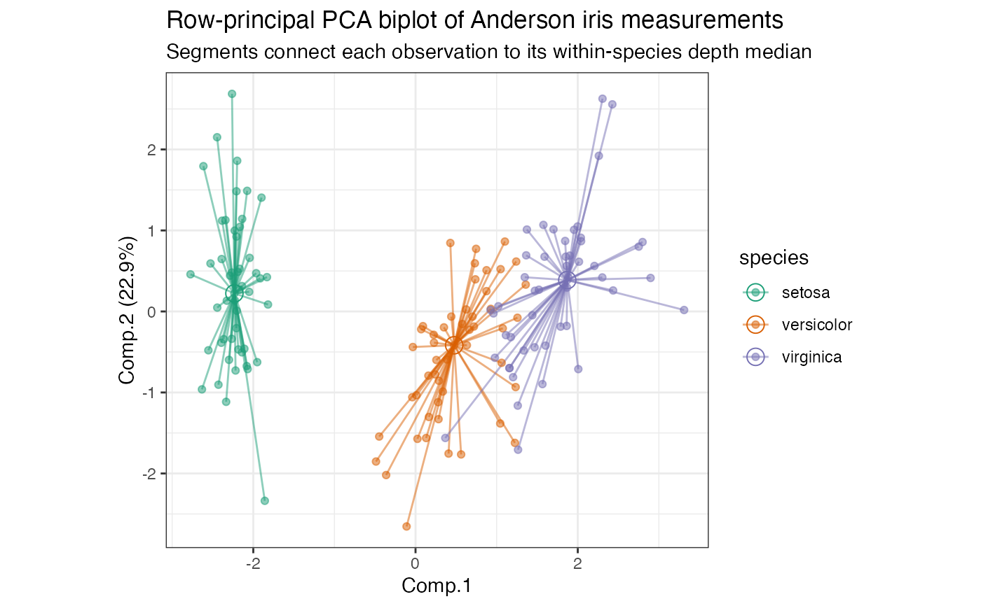
# row-principal biplot with depth median-based stars
iris_pca %>%
ggbiplot(aes(color = species)) +
theme_bw() +
scale_color_brewer(type = "qual", palette = 2) +
stat_rows_star(alpha = .5, fun.ord = "depth_median") +
geom_rows_point(alpha = .5) +
stat_rows_center(fun.ord = "depth_median", size = 4, shape = 1L) +
ggtitle(
"Row-principal PCA biplot of Anderson iris measurements",
"Segments connect each observation to its within-species depth median"
)
# scaled PCA of Anderson iris measurements
iris[, -5] %>%
princomp(cor = TRUE) %>%
as_tbl_ord() %>%
mutate_rows(species = iris$Species) %>%
print() -> iris_pca
#> # A tbl_ord of class 'princomp': (150 x 4) x (4 x 4)'
#> # 4 coordinates: Comp.1, Comp.2, ..., Comp.4
#> #
#> # Rows (principal): [ 150 x 4 | 1 ]
#> Comp.1 Comp.2 Comp.3 ... | species
#> | <fct>
#> 1 -2.26 0.480 0.128 | 1 setosa
#> 2 -2.08 -0.674 0.235 | 2 setosa
#> 3 -2.36 -0.342 -0.0442 ... | 3 setosa
#> 4 -2.30 -0.597 -0.0913 | 4 setosa
#> 5 -2.39 0.647 -0.0157 | 5 setosa
#> # ℹ 145 more rows | # ℹ 145 more rows
#>
#> #
#> # Columns (standard): [ 4 x 4 | 0 ]
#> Comp.1 Comp.2 Comp.3 ... |
#> |
#> 1 0.521 0.377 0.720 |
#> 2 -0.269 0.923 -0.244 ... |
#> 3 0.580 0.0245 -0.142 |
#> 4 0.565 0.0669 -0.634 |
# row-principal biplot with depth median-based stars
iris_pca %>%
ggbiplot(aes(color = species)) +
theme_bw() +
scale_color_brewer(type = "qual", palette = 2) +
stat_rows_star(alpha = .5, fun.ord = "depth_median") +
geom_rows_point(alpha = .5) +
stat_rows_center(fun.ord = "depth_median", size = 4, shape = 1L) +
ggtitle(
"Row-principal PCA biplot of Anderson iris measurements",
"Segments connect each observation to its within-species depth median"
)
 # correspondence analysis of combined female and male hair and eye color data
HairEyeColor %>%
rowSums(dims = 2L) %>%
MASS::corresp(nf = 2L) %>%
as_tbl_ord() %>%
augment_ord() %>%
print() -> hec_ca
#> # A tbl_ord of class 'correspondence': (4 x 2) x (4 x 2)'
#> # 2 coordinates: Can1 and Can2
#> #
#> # Rows (standard): [ 4 x 2 | 1 ]
#> Can1 Can2 | name
#> | <chr>
#> 1 -1.10 1.44 | 1 Black
#> 2 -0.324 -0.219 | 2 Brown
#> 3 -0.283 -2.14 | 3 Red
#> 4 1.83 0.467 | 4 Blond
#> #
#> # Columns (standard): [ 4 x 2 | 1 ]
#> Can1 Can2 | name
#> | <chr>
#> 1 -1.08 0.592 | 1 Brown
#> 2 1.20 0.556 | 2 Blue
#> 3 -0.465 -1.12 | 3 Hazel
#> 4 0.354 -2.27 | 4 Green
# inertia across artificial coordinates (all singular values < 1)
get_inertia(hec_ca)
#> Can1 Can2
#> 0.20877265 0.02222661
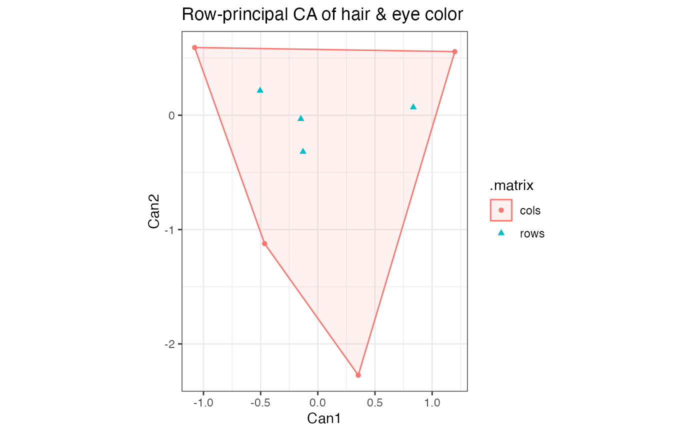
# in row-principal biplot, row coordinates are weighted averages of columns
# (and vice-versa)
hec_ca %>%
confer_inertia("rows") %>%
ggbiplot(aes(color = .matrix, fill = .matrix, shape = .matrix)) +
theme_bw() +
stat_cols_chull(alpha = .1) +
geom_cols_point() +
geom_rows_point() +
ggtitle("Row-principal CA of hair & eye color")
# correspondence analysis of combined female and male hair and eye color data
HairEyeColor %>%
rowSums(dims = 2L) %>%
MASS::corresp(nf = 2L) %>%
as_tbl_ord() %>%
augment_ord() %>%
print() -> hec_ca
#> # A tbl_ord of class 'correspondence': (4 x 2) x (4 x 2)'
#> # 2 coordinates: Can1 and Can2
#> #
#> # Rows (standard): [ 4 x 2 | 1 ]
#> Can1 Can2 | name
#> | <chr>
#> 1 -1.10 1.44 | 1 Black
#> 2 -0.324 -0.219 | 2 Brown
#> 3 -0.283 -2.14 | 3 Red
#> 4 1.83 0.467 | 4 Blond
#> #
#> # Columns (standard): [ 4 x 2 | 1 ]
#> Can1 Can2 | name
#> | <chr>
#> 1 -1.08 0.592 | 1 Brown
#> 2 1.20 0.556 | 2 Blue
#> 3 -0.465 -1.12 | 3 Hazel
#> 4 0.354 -2.27 | 4 Green
# inertia across artificial coordinates (all singular values < 1)
get_inertia(hec_ca)
#> Can1 Can2
#> 0.20877265 0.02222661
# in row-principal biplot, row coordinates are weighted averages of columns
# (and vice-versa)
hec_ca %>%
confer_inertia("rows") %>%
ggbiplot(aes(color = .matrix, fill = .matrix, shape = .matrix)) +
theme_bw() +
stat_cols_chull(alpha = .1) +
geom_cols_point() +
geom_rows_point() +
ggtitle("Row-principal CA of hair & eye color")
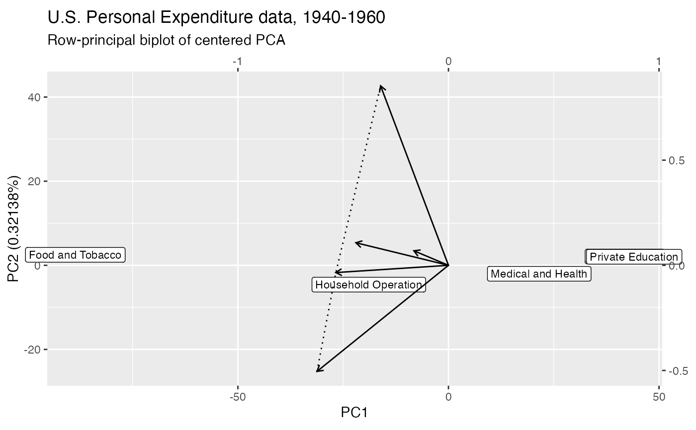
 # centered principal components analysis of U.S. personal expenditure data
USPersonalExpenditure %>%
prcomp() %>%
as_tbl_ord() %>%
augment_ord() %>%
# allow radiating text to exceed plotting window
ggbiplot(aes(label = name), clip = "off",
sec.axes = "cols", scale.factor = 50) +
geom_rows_label(size = 3) +
# omit labels in the conical hull without the origin
geom_cols_vector(vector_labels = FALSE) +
stat_cols_cone(linetype = "dotted") +
geom_cols_vector(stat = "cone", vector_labels = TRUE, color = "transparent") +
ggtitle(
"U.S. Personal Expenditure data, 1940-1960",
"Row-principal biplot of centered PCA"
)
# centered principal components analysis of U.S. personal expenditure data
USPersonalExpenditure %>%
prcomp() %>%
as_tbl_ord() %>%
augment_ord() %>%
# allow radiating text to exceed plotting window
ggbiplot(aes(label = name), clip = "off",
sec.axes = "cols", scale.factor = 50) +
geom_rows_label(size = 3) +
# omit labels in the conical hull without the origin
geom_cols_vector(vector_labels = FALSE) +
stat_cols_cone(linetype = "dotted") +
geom_cols_vector(stat = "cone", vector_labels = TRUE, color = "transparent") +
ggtitle(
"U.S. Personal Expenditure data, 1940-1960",
"Row-principal biplot of centered PCA"
)
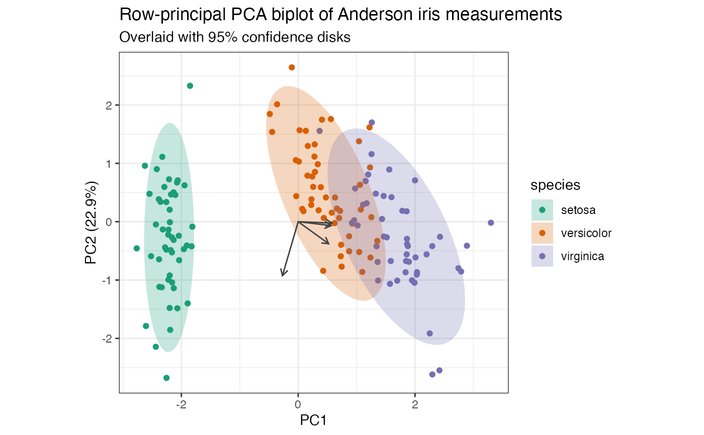
 # compute row-principal components of scaled iris measurements
iris[, -5] %>%
prcomp(scale = TRUE) %>%
as_tbl_ord() %>%
mutate_rows(species = iris$Species) %>%
print() -> iris_pca
#> # A tbl_ord of class 'prcomp': (150 x 4) x (4 x 4)'
#> # 4 coordinates: PC1, PC2, ..., PC4
#> #
#> # Rows (principal): [ 150 x 4 | 1 ]
#> PC1 PC2 PC3 ... | species
#> | <fct>
#> 1 -2.26 -0.478 0.127 | 1 setosa
#> 2 -2.07 0.672 0.234 | 2 setosa
#> 3 -2.36 0.341 -0.0441 ... | 3 setosa
#> 4 -2.29 0.595 -0.0910 | 4 setosa
#> 5 -2.38 -0.645 -0.0157 | 5 setosa
#> # ℹ 145 more rows | # ℹ 145 more rows
#>
#> #
#> # Columns (standard): [ 4 x 4 | 0 ]
#> PC1 PC2 PC3 ... |
#> |
#> 1 0.521 -0.377 0.720 |
#> 2 -0.269 -0.923 -0.244 ... |
#> 3 0.580 -0.0245 -0.142 |
#> 4 0.565 -0.0669 -0.634 |
# row-principal biplot with centroids and confidence elliptical disks
iris_pca %>%
ggbiplot(aes(color = species)) +
theme_bw() +
geom_rows_point() +
geom_polygon(
aes(fill = species),
color = NA, alpha = .25, stat = "rows_ellipse"
) +
geom_cols_vector(color = "#444444") +
scale_color_brewer(
type = "qual", palette = 2,
aesthetics = c("color", "fill")
) +
ggtitle(
"Row-principal PCA biplot of Anderson iris measurements",
"Overlaid with 95% confidence disks"
)
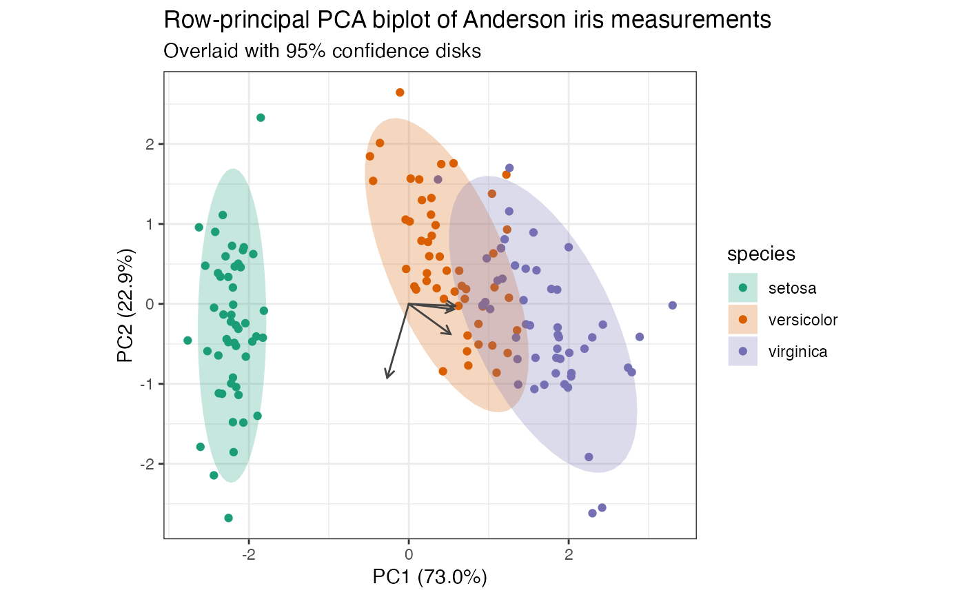
# compute row-principal components of scaled iris measurements
iris[, -5] %>%
prcomp(scale = TRUE) %>%
as_tbl_ord() %>%
mutate_rows(species = iris$Species) %>%
print() -> iris_pca
#> # A tbl_ord of class 'prcomp': (150 x 4) x (4 x 4)'
#> # 4 coordinates: PC1, PC2, ..., PC4
#> #
#> # Rows (principal): [ 150 x 4 | 1 ]
#> PC1 PC2 PC3 ... | species
#> | <fct>
#> 1 -2.26 -0.478 0.127 | 1 setosa
#> 2 -2.07 0.672 0.234 | 2 setosa
#> 3 -2.36 0.341 -0.0441 ... | 3 setosa
#> 4 -2.29 0.595 -0.0910 | 4 setosa
#> 5 -2.38 -0.645 -0.0157 | 5 setosa
#> # ℹ 145 more rows | # ℹ 145 more rows
#>
#> #
#> # Columns (standard): [ 4 x 4 | 0 ]
#> PC1 PC2 PC3 ... |
#> |
#> 1 0.521 -0.377 0.720 |
#> 2 -0.269 -0.923 -0.244 ... |
#> 3 0.580 -0.0245 -0.142 |
#> 4 0.565 -0.0669 -0.634 |
# row-principal biplot with centroids and confidence elliptical disks
iris_pca %>%
ggbiplot(aes(color = species)) +
theme_bw() +
geom_rows_point() +
geom_polygon(
aes(fill = species),
color = NA, alpha = .25, stat = "rows_ellipse"
) +
geom_cols_vector(color = "#444444") +
scale_color_brewer(
type = "qual", palette = 2,
aesthetics = c("color", "fill")
) +
ggtitle(
"Row-principal PCA biplot of Anderson iris measurements",
"Overlaid with 95% confidence disks"
)
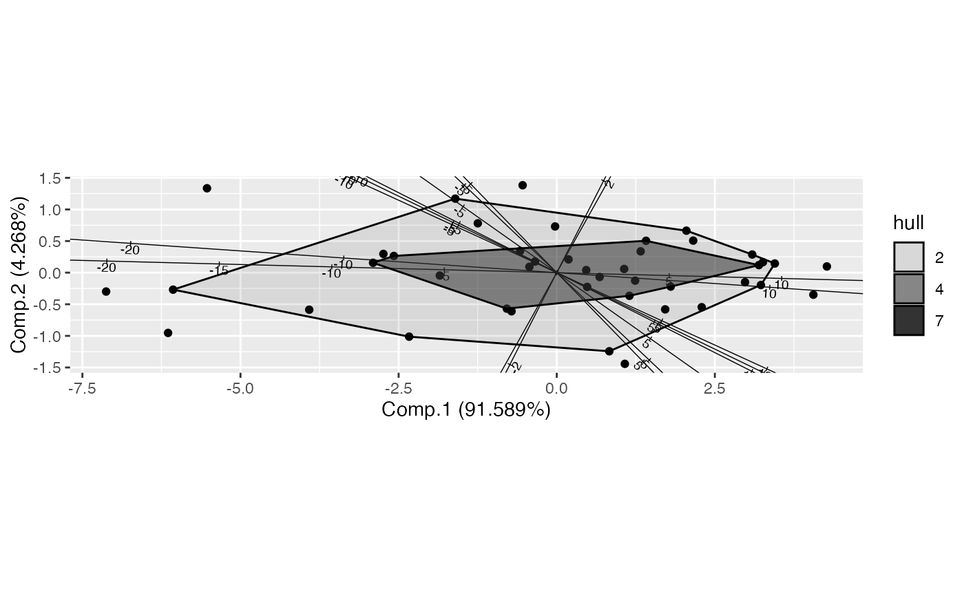
 # hull peeling with breaks below
judge_pca <- ordinate(USJudgeRatings, princomp, cols = -c(1, 12))
ggbiplot(judge_pca, axis.type = "predictive") +
geom_cols_axis() +
geom_rows_point(elements = "score") +
stat_rows_peel(
aes(alpha = after_stat(hull)), color = "black", elements = "score",
breaks = c(.9, .5, .1), cut = "below"
)
#> Warning: Using alpha for a discrete variable is not advised.
# hull peeling with breaks below
judge_pca <- ordinate(USJudgeRatings, princomp, cols = -c(1, 12))
ggbiplot(judge_pca, axis.type = "predictive") +
geom_cols_axis() +
geom_rows_point(elements = "score") +
stat_rows_peel(
aes(alpha = after_stat(hull)), color = "black", elements = "score",
breaks = c(.9, .5, .1), cut = "below"
)
#> Warning: Using alpha for a discrete variable is not advised.
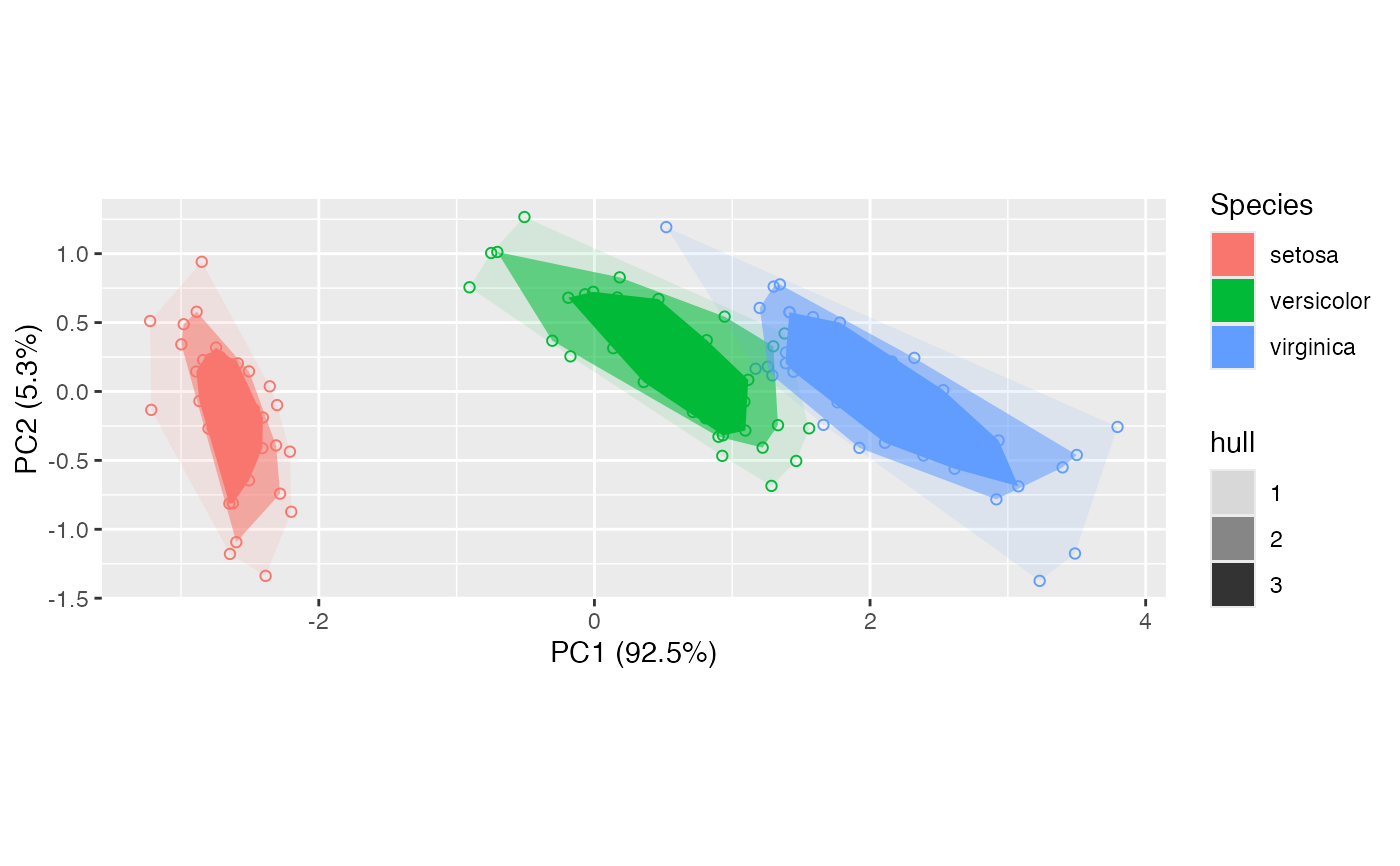
 # hull peeling by groups
iris_pca <- ordinate(iris, cols = 1:4, model = prcomp)
ggbiplot(iris_pca) +
geom_rows_point(aes(color = Species), shape = "circle open") +
stat_rows_peel(
aes(fill = Species, alpha = after_stat(hull)),
num = 3
)
#> Warning: Using alpha for a discrete variable is not advised.
# hull peeling by groups
iris_pca <- ordinate(iris, cols = 1:4, model = prcomp)
ggbiplot(iris_pca) +
geom_rows_point(aes(color = Species), shape = "circle open") +
stat_rows_peel(
aes(fill = Species, alpha = after_stat(hull)),
num = 3
)
#> Warning: Using alpha for a discrete variable is not advised.
 # unscaled PCA
iris_pca <- ordinate(iris, cols = 1:4, model = prcomp)
# biplot canvas
iris_biplot <-
iris_pca %>%
ggbiplot(aes(color = Species, label = name), axis.type = "predictive") +
geom_rows_point() +
geom_cols_axis(aes(center = center))
# print select cases
top_cases <- c(1, 51, 101)
iris[top_cases, ]
#> Sepal.Length Sepal.Width Petal.Length Petal.Width Species
#> 1 5.1 3.5 1.4 0.2 setosa
#> 51 7.0 3.2 4.7 1.4 versicolor
#> 101 6.3 3.3 6.0 2.5 virginica
# subset variables
length_vars <- c(1, 3)
iris[, length_vars] %>%
aggregate(by = iris[, "Species", drop = FALSE], FUN = mean)
#> Species Sepal.Length Petal.Length
#> 1 setosa 5.006 1.462
#> 2 versicolor 5.936 4.260
#> 3 virginica 6.588 5.552
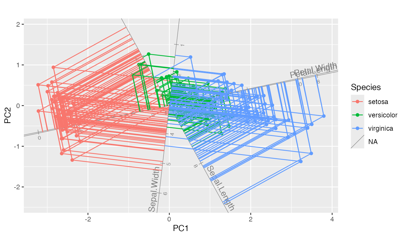
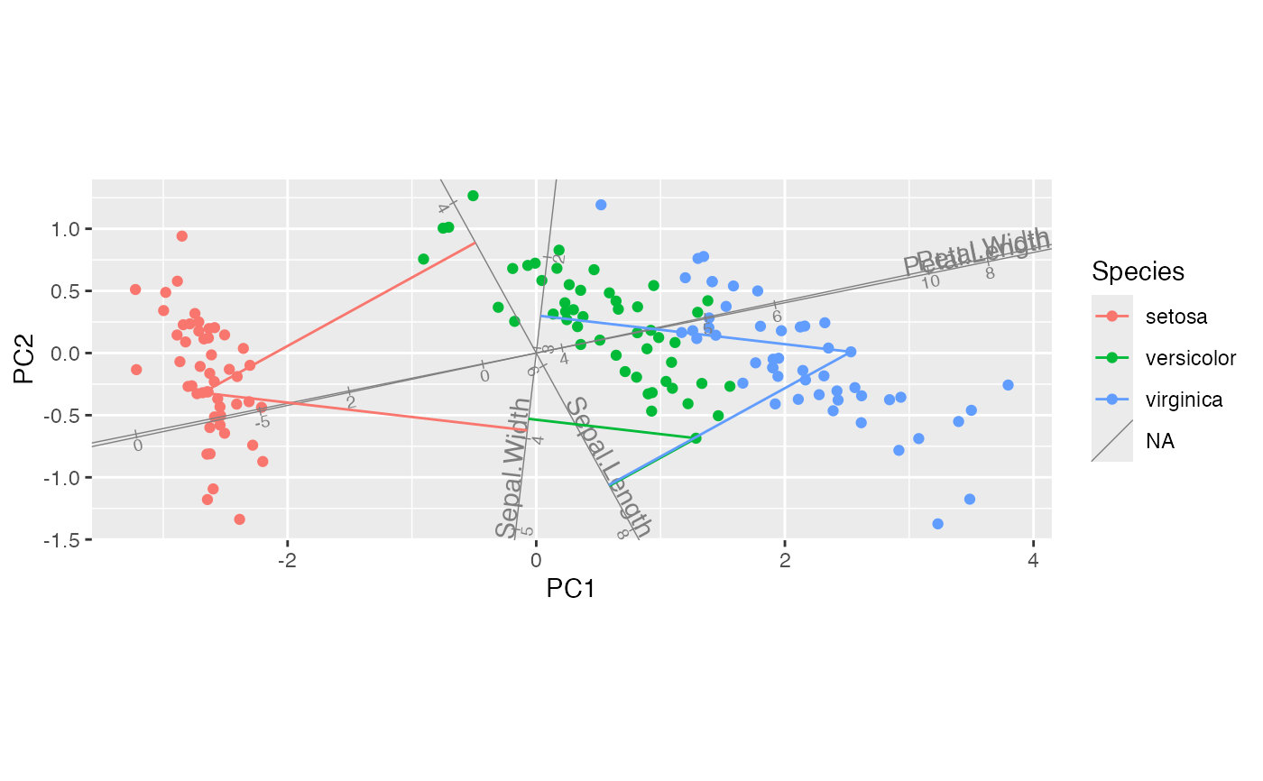
# project all cases onto all axes
iris_biplot + stat_rows_projection()
# unscaled PCA
iris_pca <- ordinate(iris, cols = 1:4, model = prcomp)
# biplot canvas
iris_biplot <-
iris_pca %>%
ggbiplot(aes(color = Species, label = name), axis.type = "predictive") +
geom_rows_point() +
geom_cols_axis(aes(center = center))
# print select cases
top_cases <- c(1, 51, 101)
iris[top_cases, ]
#> Sepal.Length Sepal.Width Petal.Length Petal.Width Species
#> 1 5.1 3.5 1.4 0.2 setosa
#> 51 7.0 3.2 4.7 1.4 versicolor
#> 101 6.3 3.3 6.0 2.5 virginica
# subset variables
length_vars <- c(1, 3)
iris[, length_vars] %>%
aggregate(by = iris[, "Species", drop = FALSE], FUN = mean)
#> Species Sepal.Length Petal.Length
#> 1 setosa 5.006 1.462
#> 2 versicolor 5.936 4.260
#> 3 virginica 6.588 5.552
# project all cases onto all axes
iris_biplot + stat_rows_projection()
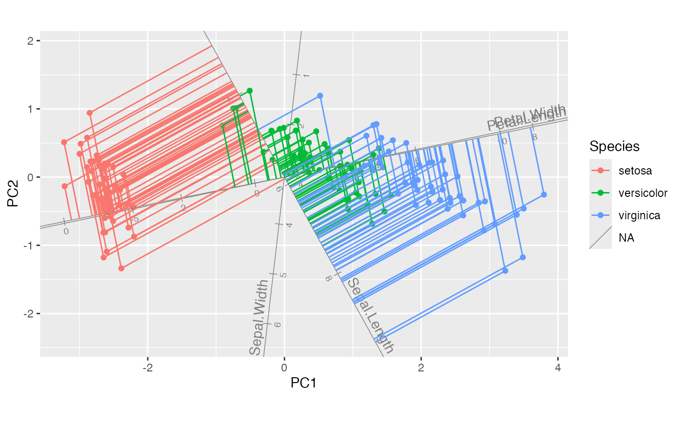
 # project all cases onto select axes
iris_biplot + stat_rows_projection(ref_subset = length_vars)
#> `subset` will be applied after data are restricted to active elements.
#> This message is displayed once per session.
# project all cases onto select axes
iris_biplot + stat_rows_projection(ref_subset = length_vars)
#> `subset` will be applied after data are restricted to active elements.
#> This message is displayed once per session.
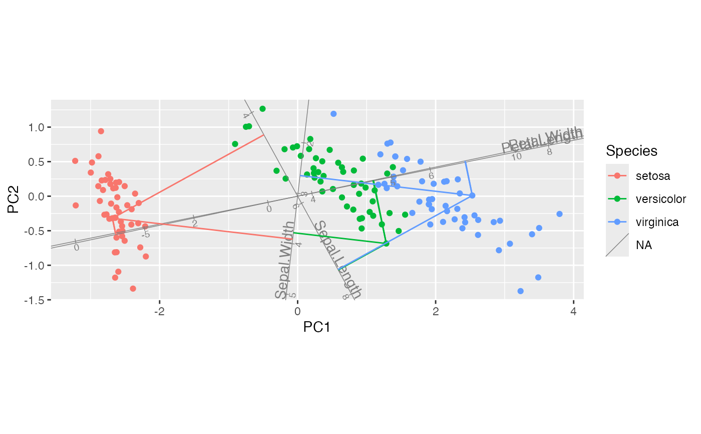
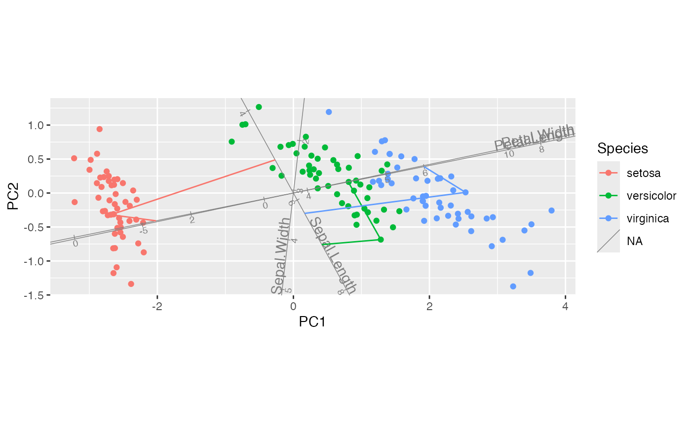
 # project select cases onto all axes
iris_biplot + stat_rows_projection(subset = top_cases)
# project select cases onto all axes
iris_biplot + stat_rows_projection(subset = top_cases)
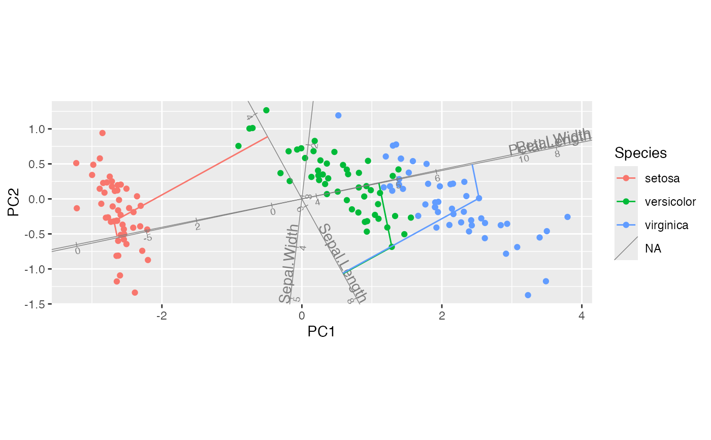
 # project select cases onto select axes
iris_biplot + stat_rows_projection(subset = top_cases, ref_subset = length_vars)
# project select cases onto select axes
iris_biplot + stat_rows_projection(subset = top_cases, ref_subset = length_vars)
 # project select cases onto manually provided axes
iris_cols <- as.data.frame(get_cols(iris_pca))[c(1, 2), ]
iris_biplot + stat_rows_projection(subset = top_cases, referent = iris_cols)
# project select cases onto manually provided axes
iris_cols <- as.data.frame(get_cols(iris_pca))[c(1, 2), ]
iris_biplot + stat_rows_projection(subset = top_cases, referent = iris_cols)
 # project selected cases onto selected axes in full-dimensional space
iris_pca %>%
ggbiplot(ord_aes(iris_pca, color = Species, label = name),
axis.type = "predictive") +
geom_rows_point() +
geom_cols_axis(aes(center = center)) +
stat_rows_projection(subset = top_cases, ref_subset = length_vars)
# project selected cases onto selected axes in full-dimensional space
iris_pca %>%
ggbiplot(ord_aes(iris_pca, color = Species, label = name),
axis.type = "predictive") +
geom_rows_point() +
geom_cols_axis(aes(center = center)) +
stat_rows_projection(subset = top_cases, ref_subset = length_vars)
 # default (standardized) linear discriminant analysis
glass_lda <- MASS::lda(Site ~ SiO2 + Al2O3 + FeO + MgO + CaO, glass)
# bestow 'tbl_ord' class & augment observation, centroid, and variable fields
as_tbl_ord(glass_lda) %>%
augment_ord() %>%
print() -> glass_lda
#> # A tbl_ord of class 'lda': (72 x 3) x (5 x 3)'
#> # 3 coordinates: LD1, LD2, LD3
#> #
#> # Rows (principal): [ 72 x 3 | 5 ]
#> LD1 LD2 LD3 | name prior counts grouping
#> | <chr> <dbl> <int> <chr>
#> 1 1.82 -1.21 -0.672 | 1 Apollonia 0.132 9 Apollon…
#> 2 -5.62 0.364 -0.00398 | 2 Banias 0.265 18 Banias
#> 3 2.47 1.63 0.0833 | 3 Bet Eli'ez… 0.397 27 Bet Eli…
#> 4 1.31 -2.84 0.277 | 4 Dor 0.206 14 Dor
#> 5 2.99 2.03 -1.22 | 5 1 NA NA Bet Eli…
#> # ℹ 67 more rows | # ℹ 67 more rows
#> # ℹ 1 more variable: .element <chr>
#> #
#> # Columns (standard): [ 5 x 3 | 2 ]
#> LD1 LD2 LD3 | name .element
#> | <chr> <chr>
#> 1 0.00681 0.618 0.468 | 1 SiO2 active
#> 2 2.05 1.04 -0.660 | 2 Al2O3 active
#> 3 -1.93 0.165 2.44 | 3 FeO active
#> 4 -1.76 1.82 -0.599 | 4 MgO active
#> 5 -0.275 0.0942 1.42 | 5 CaO active
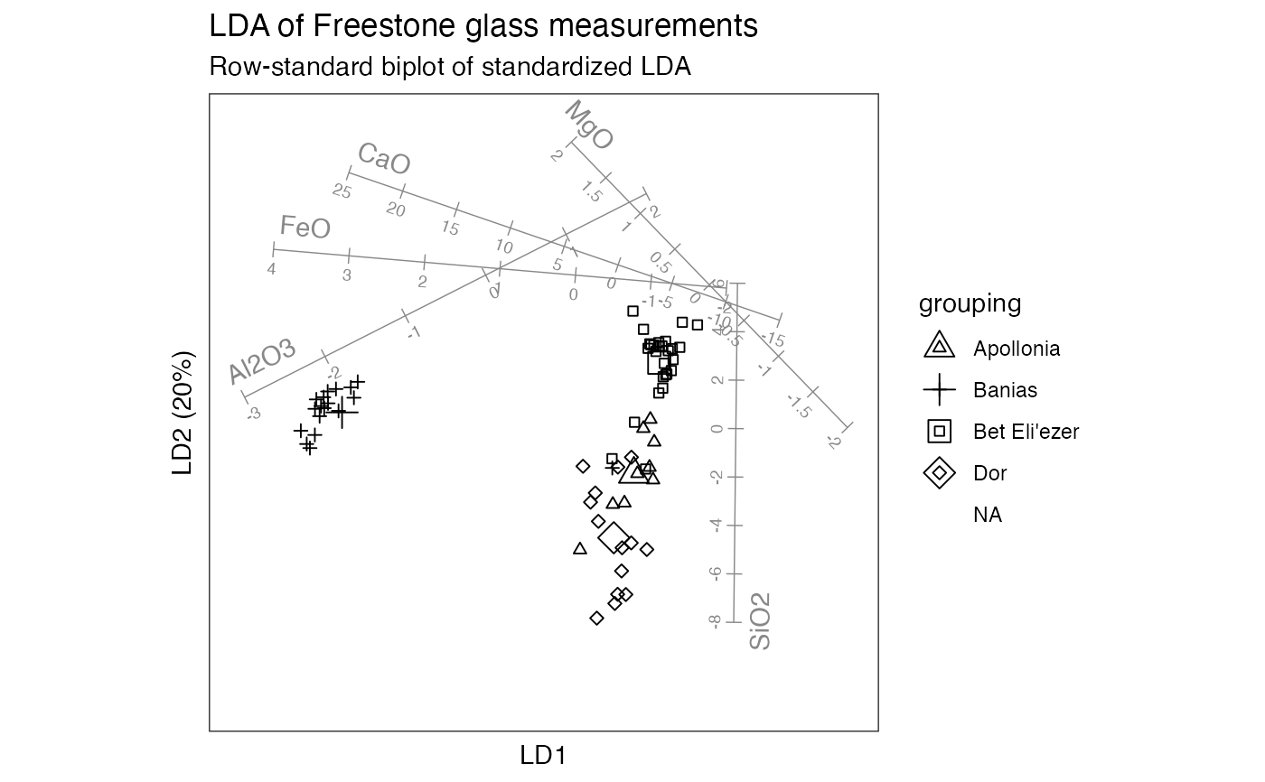
# row-standard biplot
glass_lda %>%
confer_inertia(1) %>%
ggbiplot(aes(shape = grouping)) +
theme_bw() + theme_biplot() +
geom_rows_point(size = 4) +
geom_rows_point(elements = "score") +
stat_cols_rule(
aes(label = name), color = "#888888", num = 8L,
ref_elements = "score", fun.offset = function(x) minabspp(x, p = .1),
text.size = 2.5, label_dodge = .04
) +
scale_shape_manual(values = c(2L, 3L, 0L, 5L)) +
ggtitle(
"LDA of Freestone glass measurements",
"Row-standard biplot of standardized LDA"
)
# default (standardized) linear discriminant analysis
glass_lda <- MASS::lda(Site ~ SiO2 + Al2O3 + FeO + MgO + CaO, glass)
# bestow 'tbl_ord' class & augment observation, centroid, and variable fields
as_tbl_ord(glass_lda) %>%
augment_ord() %>%
print() -> glass_lda
#> # A tbl_ord of class 'lda': (72 x 3) x (5 x 3)'
#> # 3 coordinates: LD1, LD2, LD3
#> #
#> # Rows (principal): [ 72 x 3 | 5 ]
#> LD1 LD2 LD3 | name prior counts grouping
#> | <chr> <dbl> <int> <chr>
#> 1 1.82 -1.21 -0.672 | 1 Apollonia 0.132 9 Apollon…
#> 2 -5.62 0.364 -0.00398 | 2 Banias 0.265 18 Banias
#> 3 2.47 1.63 0.0833 | 3 Bet Eli'ez… 0.397 27 Bet Eli…
#> 4 1.31 -2.84 0.277 | 4 Dor 0.206 14 Dor
#> 5 2.99 2.03 -1.22 | 5 1 NA NA Bet Eli…
#> # ℹ 67 more rows | # ℹ 67 more rows
#> # ℹ 1 more variable: .element <chr>
#> #
#> # Columns (standard): [ 5 x 3 | 2 ]
#> LD1 LD2 LD3 | name .element
#> | <chr> <chr>
#> 1 0.00681 0.618 0.468 | 1 SiO2 active
#> 2 2.05 1.04 -0.660 | 2 Al2O3 active
#> 3 -1.93 0.165 2.44 | 3 FeO active
#> 4 -1.76 1.82 -0.599 | 4 MgO active
#> 5 -0.275 0.0942 1.42 | 5 CaO active
# row-standard biplot
glass_lda %>%
confer_inertia(1) %>%
ggbiplot(aes(shape = grouping)) +
theme_bw() + theme_biplot() +
geom_rows_point(size = 4) +
geom_rows_point(elements = "score") +
stat_cols_rule(
aes(label = name), color = "#888888", num = 8L,
ref_elements = "score", fun.offset = function(x) minabspp(x, p = .1),
text.size = 2.5, label_dodge = .04
) +
scale_shape_manual(values = c(2L, 3L, 0L, 5L)) +
ggtitle(
"LDA of Freestone glass measurements",
"Row-standard biplot of standardized LDA"
)
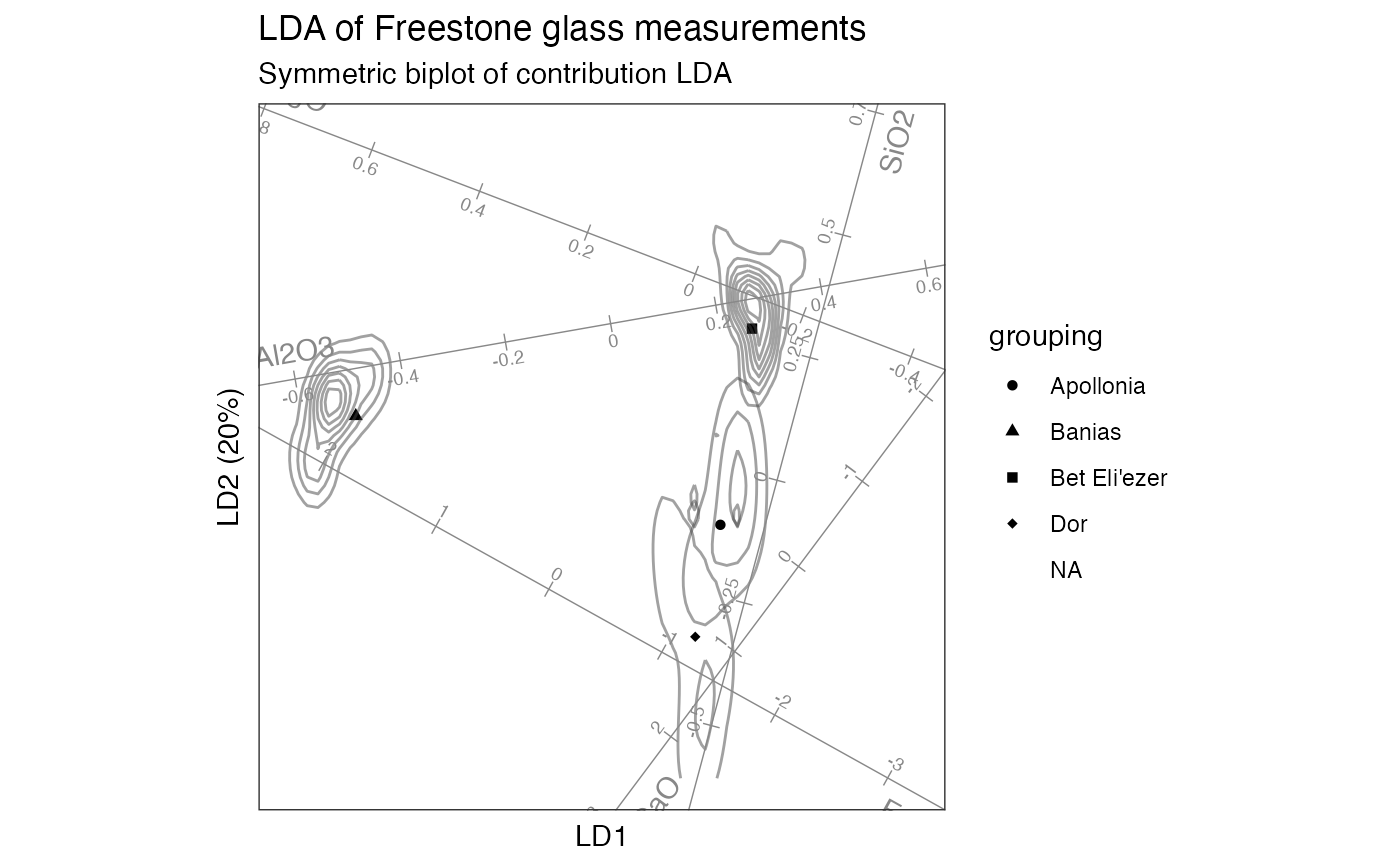
 # contribution LDA of sites on measurements
glass_lda <-
lda_ord(Site ~ SiO2 + Al2O3 + FeO + MgO + CaO, glass,
axes.scale = "contribution")
# bestow 'tbl_ord' class & augment observation, centroid, and variable fields
as_tbl_ord(glass_lda) %>%
augment_ord() %>%
print() -> glass_lda
#> # A tbl_ord of class 'lda_ord': (72 x 3) x (5 x 3)'
#> # 3 coordinates: LD1, LD2, LD3
#> #
#> # Rows (principal): [ 72 x 3 | 5 ]
#> LD1 LD2 LD3 | name prior counts grouping
#> | <chr> <dbl> <int> <chr>
#> 1 1.82 -1.21 -0.672 | 1 Apollonia 0.132 9 Apollon…
#> 2 -5.62 0.364 -0.00398 | 2 Banias 0.265 18 Banias
#> 3 2.47 1.63 0.0833 | 3 Bet Eli'ez… 0.397 27 Bet Eli…
#> 4 1.31 -2.84 0.277 | 4 Dor 0.206 14 Dor
#> 5 2.99 2.03 -1.22 | 5 1 NA NA Bet Eli…
#> # ℹ 67 more rows | # ℹ 67 more rows
#> # ℹ 1 more variable: .element <chr>
#> #
#> # Columns (standard): [ 5 x 3 | 2 ]
#> LD1 LD2 LD3 | name .element
#> | <chr> <chr>
#> 1 0.166 0.871 0.160 | 1 SiO2 active
#> 2 0.663 0.164 0.0442 | 2 Al2O3 active
#> 3 -0.142 0.112 0.192 | 3 FeO active
#> 4 -0.680 0.367 -0.0694 | 4 MgO active
#> 5 -0.0804 -0.151 0.941 | 5 CaO active
# symmetric biplot
glass_lda %>%
confer_inertia(.5) %>%
ggbiplot(aes(shape = grouping)) +
theme_bw() + theme_biplot() +
geom_rows_point() +
stat_rows_density_2d(elements = "score", alpha = .5, color = "#444444") +
stat_cols_rule(
aes(label = name), geom = "axis", color = "#888888", num = 8L,
ref_elements = "active", fun.offset = function(x) minabspp(x, p = .1),
label_dodge = 0.04, text.size = 2.5, text_dodge = .025
) +
scale_shape_manual(values = c(16L, 17L, 15L, 18L)) +
ggtitle(
"LDA of Freestone glass measurements",
"Symmetric biplot of contribution LDA"
)
# contribution LDA of sites on measurements
glass_lda <-
lda_ord(Site ~ SiO2 + Al2O3 + FeO + MgO + CaO, glass,
axes.scale = "contribution")
# bestow 'tbl_ord' class & augment observation, centroid, and variable fields
as_tbl_ord(glass_lda) %>%
augment_ord() %>%
print() -> glass_lda
#> # A tbl_ord of class 'lda_ord': (72 x 3) x (5 x 3)'
#> # 3 coordinates: LD1, LD2, LD3
#> #
#> # Rows (principal): [ 72 x 3 | 5 ]
#> LD1 LD2 LD3 | name prior counts grouping
#> | <chr> <dbl> <int> <chr>
#> 1 1.82 -1.21 -0.672 | 1 Apollonia 0.132 9 Apollon…
#> 2 -5.62 0.364 -0.00398 | 2 Banias 0.265 18 Banias
#> 3 2.47 1.63 0.0833 | 3 Bet Eli'ez… 0.397 27 Bet Eli…
#> 4 1.31 -2.84 0.277 | 4 Dor 0.206 14 Dor
#> 5 2.99 2.03 -1.22 | 5 1 NA NA Bet Eli…
#> # ℹ 67 more rows | # ℹ 67 more rows
#> # ℹ 1 more variable: .element <chr>
#> #
#> # Columns (standard): [ 5 x 3 | 2 ]
#> LD1 LD2 LD3 | name .element
#> | <chr> <chr>
#> 1 0.166 0.871 0.160 | 1 SiO2 active
#> 2 0.663 0.164 0.0442 | 2 Al2O3 active
#> 3 -0.142 0.112 0.192 | 3 FeO active
#> 4 -0.680 0.367 -0.0694 | 4 MgO active
#> 5 -0.0804 -0.151 0.941 | 5 CaO active
# symmetric biplot
glass_lda %>%
confer_inertia(.5) %>%
ggbiplot(aes(shape = grouping)) +
theme_bw() + theme_biplot() +
geom_rows_point() +
stat_rows_density_2d(elements = "score", alpha = .5, color = "#444444") +
stat_cols_rule(
aes(label = name), geom = "axis", color = "#888888", num = 8L,
ref_elements = "active", fun.offset = function(x) minabspp(x, p = .1),
label_dodge = 0.04, text.size = 2.5, text_dodge = .025
) +
scale_shape_manual(values = c(16L, 17L, 15L, 18L)) +
ggtitle(
"LDA of Freestone glass measurements",
"Symmetric biplot of contribution LDA"
)
 if (FALSE) { # \dontrun{
# classical multidimensional scaling of road distances between European cities
euro_mds <- ordinate(eurodist, cmdscale_ord, k = 11)
# monoplot of city locations
euro_plot <- euro_mds %>%
negate_ord("PCo2") %>%
ggbiplot() +
geom_cols_text(aes(label = name), size = 3)
print(euro_plot)
# biplot with minimal spanning tree based on plotting window distances
euro_plot +
stat_cols_spantree(
engine = "mlpack",
alpha = .5, linetype = "dotted"
)
# biplot with minimal spanning tree based on full-dimensional distances
euro_plot +
stat_cols_spantree(
ord_aes(euro_mds), engine = "mlpack",
alpha = .5, linetype = "dotted"
)
} # }
if (FALSE) { # \dontrun{
# classical multidimensional scaling of road distances between European cities
euro_mds <- ordinate(eurodist, cmdscale_ord, k = 11)
# monoplot of city locations
euro_plot <- euro_mds %>%
negate_ord("PCo2") %>%
ggbiplot() +
geom_cols_text(aes(label = name), size = 3)
print(euro_plot)
# biplot with minimal spanning tree based on plotting window distances
euro_plot +
stat_cols_spantree(
engine = "mlpack",
alpha = .5, linetype = "dotted"
)
# biplot with minimal spanning tree based on full-dimensional distances
euro_plot +
stat_cols_spantree(
ord_aes(euro_mds), engine = "mlpack",
alpha = .5, linetype = "dotted"
)
} # }