geom_axis() renders lines through or orthogonally translated
from the origin and the position of each case or variable.
Usage
geom_axis(
  mapping = NULL,
  data = NULL,
  stat = "identity",
  position = "identity",
  axis_labels = TRUE,
  axis_ticks = TRUE,
  axis_text = TRUE,
  by = NULL,
  num = NULL,
  tick_length = 0.025,
  text_dodge = 0.03,
  label_dodge = 0.03,
  ...,
  axis.colour = NULL,
  axis.color = NULL,
  axis.alpha = NULL,
  label.angle = 0,
  label.colour = NULL,
  label.color = NULL,
  label.alpha = NULL,
  tick.linewidth = 0.25,
  tick.colour = NULL,
  tick.color = NULL,
  tick.alpha = NULL,
  text.size = 2.6,
  text.angle = 0,
  text.hjust = 0.5,
  text.vjust = 0.5,
  text.family = NULL,
  text.fontface = NULL,
  text.colour = NULL,
  text.color = NULL,
  text.alpha = NULL,
  parse = FALSE,
  check_overlap = FALSE,
  na.rm = FALSE,
  show.legend = NA,
  inherit.aes = TRUE
)
Arguments
- mapping
Set of aesthetic mappings created by
aes(). If specified andinherit.aes = TRUE(the default), it is combined with the default mapping at the top level of the plot. You must supplymappingif there is no plot mapping.- data
The data to be displayed in this layer. There are three options:
If
NULL, the default, the data is inherited from the plot data as specified in the call toggplot().A
data.frame, or other object, will override the plot data. All objects will be fortified to produce a data frame. Seefortify()for which variables will be created.A
functionwill be called with a single argument, the plot data. The return value must be adata.frame, and will be used as the layer data. Afunctioncan be created from aformula(e.g.~ head(.x, 10)).- stat
The statistical transformation to use on the data for this layer. When using a
geom_*()function to construct a layer, thestatargument can be used the override the default coupling between geoms and stats. Thestatargument accepts the following:A
Statggproto subclass, for exampleStatCount.A string naming the stat. To give the stat as a string, strip the function name of the
stat_prefix. For example, to usestat_count(), give the stat as"count".For more information and other ways to specify the stat, see the layer stat documentation.
- position
A position adjustment to use on the data for this layer. This can be used in various ways, including to prevent overplotting and improving the display. The
positionargument accepts the following:The result of calling a position function, such as
position_jitter(). This method allows for passing extra arguments to the position.A string naming the position adjustment. To give the position as a string, strip the function name of the
position_prefix. For example, to useposition_jitter(), give the position as"jitter".For more information and other ways to specify the position, see the layer position documentation.
- axis_labels, axis_ticks, axis_text
Logical; whether to include labels, tick marks, and text value marks along the axes.
- by, num
Intervals between elements or number of elements; specify only one.
- tick_length
Numeric; the length of the tick marks, as a proportion of the minimum of the plot width and height.
- text_dodge
Numeric; the orthogonal distance of tick mark text from the axis, as a proportion of the minimum of the plot width and height.
- label_dodge
Numeric; the orthogonal distance of the axis label from the axis, as a proportion of the minimum of the plot width and height.
- ...
Additional arguments passed to
ggplot2::layer().- axis.colour, axis.color, axis.alpha
Default aesthetics for axes. Set to NULL to inherit from the data's aesthetics.
- label.angle, label.colour, label.color, label.alpha
Default aesthetics for labels. Set to NULL to inherit from the data's aesthetics.
- tick.linewidth, tick.colour, tick.color, tick.alpha
Default aesthetics for tick marks. Set to NULL to inherit from the data's aesthetics.
- text.size, text.angle, text.hjust, text.vjust, text.family, text.fontface, text.colour, text.color, text.alpha
Default aesthetics for tick mark labels. Set to NULL to inherit from the data's aesthetics.
- parse
If
TRUE, the labels will be parsed into expressions and displayed as described in?plotmath.- check_overlap
If
TRUE, text that overlaps previous text in the same layer will not be plotted.check_overlaphappens at draw time and in the order of the data. Therefore data should be arranged by the label column before callinggeom_text(). Note that this argument is not supported bygeom_label().- na.rm
Passed to
ggplot2::layer().- show.legend
logical. Should this layer be included in the legends?
NA, the default, includes if any aesthetics are mapped.FALSEnever includes, andTRUEalways includes. It can also be a named logical vector to finely select the aesthetics to display.- inherit.aes
If
FALSE, overrides the default aesthetics, rather than combining with them. This is most useful for helper functions that define both data and aesthetics and shouldn't inherit behaviour from the default plot specification, e.g.borders().
Value
A ggproto layer.
Details
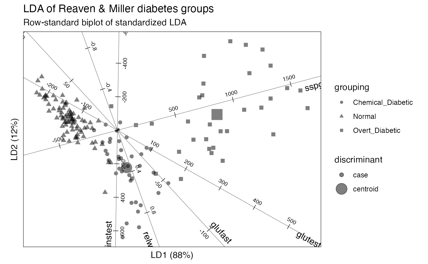
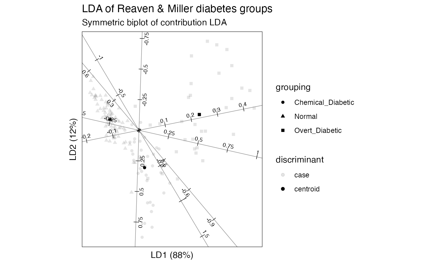
Axes are lines that track the values of linear variables across a plot. Multivariate scatterplots may include more axes than plotting dimensions, in which case the plot may display only a fraction of the total variation in the data.
Gower & Hand (1996) recommend using axes to represent numerical variables in biplots. Consequently, Gardner & le Roux (2002) refer to these as Gower biplots.
Axes positioned orthogonally at the origin are a ubiquitous feature of
scatterplots and used both to recover variable values from case markers
(prediction) and to position new case markers from variables
(interpolation). When they are not orthogonal, these two uses conflict, so
interpolative versus predictive axes must be used appropriately; see
ggbiplot().
Biplot layers
ggbiplot() uses ggplot2::fortify() internally to produce a single data
frame with a .matrix column distinguishing the subjects ("rows") and
variables ("cols"). The stat layers stat_rows() and stat_cols() simply
filter the data frame to one of these two.
The geom layers geom_rows_*() and geom_cols_*() call the corresponding
stat in order to render plot elements for the corresponding factor matrix.
geom_dims_*() selects a default matrix based on common practice, e.g.
points for rows and arrows for columns.
Aesthetics
geom_axis() understands the following aesthetics (required aesthetics are
in bold):
xylowerupperyinterceptorxinterceptorxendandyendlinetypelinewidthsizehjustvjustcolouralphalabelfamilyfontfacecenter,scalegroup
References
Gower JC & Hand DJ (1996) Biplots. Chapman & Hall, ISBN: 0-412-71630-5.
Gardner S, le Roux N (2002) "Biplot Methodology for Discriminant Analysis Based upon Robust Methods and Principal Curves". Classification, Clustering, and Data Analysis: Recent Advances and Applications: 169–176. https://link.springer.com/chapter/10.1007/978-3-642-56181-8_18
See also
Other geom layers:
geom_bagplot(),
geom_interpolation(),
geom_isoline(),
geom_lineranges(),
geom_origin(),
geom_rule(),
geom_text_radiate(),
geom_vector()
Examples
# stack loss gradient
stackloss |>
lm(formula = stack.loss ~ Air.Flow + Water.Temp + Acid.Conc.) |>
coef() |>
as.list() |> as.data.frame() |>
subset(select = c(Air.Flow, Water.Temp, Acid.Conc.)) ->
coef_data
# gradient axis with respect to two predictors
scale(stackloss, scale = FALSE) |>
ggplot(aes(x = Acid.Conc., y = Air.Flow)) +
coord_square() + geom_origin() +
geom_point(aes(size = stack.loss, alpha = sign(stack.loss))) +
scale_size_area() + scale_alpha_binned(breaks = c(-1, 0, 1)) +
geom_axis(data = coef_data)
 # unlimited axes with window forcing
stackloss_centered <- scale(stackloss, scale = FALSE)
stackloss_centered |>
ggplot(aes(x = Acid.Conc., y = Air.Flow)) +
coord_square() + geom_origin() +
geom_point(aes(size = stack.loss, alpha = sign(stack.loss))) +
scale_size_area() + scale_alpha_binned(breaks = c(-1, 0, 1)) +
stat_rule(
geom = "axis", data = coef_data,
referent = stackloss_centered,
fun.lower = \(x) minpp(x, p = 1), fun.upper = \(x) maxpp(x, p = 1),
fun.offset = \(x) minabspp(x, p = 1)
)
# unlimited axes with window forcing
stackloss_centered <- scale(stackloss, scale = FALSE)
stackloss_centered |>
ggplot(aes(x = Acid.Conc., y = Air.Flow)) +
coord_square() + geom_origin() +
geom_point(aes(size = stack.loss, alpha = sign(stack.loss))) +
scale_size_area() + scale_alpha_binned(breaks = c(-1, 0, 1)) +
stat_rule(
geom = "axis", data = coef_data,
referent = stackloss_centered,
fun.lower = \(x) minpp(x, p = 1), fun.upper = \(x) maxpp(x, p = 1),
fun.offset = \(x) minabspp(x, p = 1)
)
 # NB: `geom_axis(stat = "rule")` would fail to pass positional aesthetics.
# eigen-decomposition of covariance matrix
ability.cov$cov |>
cov2cor() |>
eigen() |> getElement("vectors") |>
as.data.frame() |>
transform(test = rownames(ability.cov$cov)) ->
ability_cor_eigen
# test axes in best-approximation space
ability_cor_eigen |>
transform(E3 = ifelse(V3 > 0, "rise", "fall")) |>
ggplot(aes(V1, V2, color = E3)) +
coord_square() +
geom_axis(aes(label = test), text.color = "black", text.alpha = .5) +
expand_limits(x = c(-1, 1), y = c(-1, 1))
# NB: `geom_axis(stat = "rule")` would fail to pass positional aesthetics.
# eigen-decomposition of covariance matrix
ability.cov$cov |>
cov2cor() |>
eigen() |> getElement("vectors") |>
as.data.frame() |>
transform(test = rownames(ability.cov$cov)) ->
ability_cor_eigen
# test axes in best-approximation space
ability_cor_eigen |>
transform(E3 = ifelse(V3 > 0, "rise", "fall")) |>
ggplot(aes(V1, V2, color = E3)) +
coord_square() +
geom_axis(aes(label = test), text.color = "black", text.alpha = .5) +
expand_limits(x = c(-1, 1), y = c(-1, 1))
