Calculate a minimum spanning tree among cases or variables
Source:R/stat-spantree.r
stat_spantree.RdThis stat layer identifies the \(n-1\) pairs among \(n\)
points that form a minimum spanning tree, then calculates the segments
between these poirs in the two dimensions x and y.
Usage
stat_spantree(
  mapping = NULL,
  data = NULL,
  geom = "segment",
  position = "identity",
  engine = "mlpack",
  method = "euclidean",
  show.legend = NA,
  inherit.aes = TRUE,
  ...
)
Arguments
- mapping
Set of aesthetic mappings created by
aes(). If specified andinherit.aes = TRUE(the default), it is combined with the default mapping at the top level of the plot. You must supplymappingif there is no plot mapping.- data
The data to be displayed in this layer. There are three options:
If
NULL, the default, the data is inherited from the plot data as specified in the call toggplot().A
data.frame, or other object, will override the plot data. All objects will be fortified to produce a data frame. Seefortify()for which variables will be created.A
functionwill be called with a single argument, the plot data. The return value must be adata.frame, and will be used as the layer data. Afunctioncan be created from aformula(e.g.~ head(.x, 10)).- geom
The geometric object to use to display the data for this layer. When using a
stat_*()function to construct a layer, thegeomargument can be used to override the default coupling between stats and geoms. Thegeomargument accepts the following:A
Geomggproto subclass, for exampleGeomPoint.A string naming the geom. To give the geom as a string, strip the function name of the
geom_prefix. For example, to usegeom_point(), give the geom as"point".For more information and other ways to specify the geom, see the layer geom documentation.
- position
A position adjustment to use on the data for this layer. This can be used in various ways, including to prevent overplotting and improving the display. The
positionargument accepts the following:The result of calling a position function, such as
position_jitter(). This method allows for passing extra arguments to the position.A string naming the position adjustment. To give the position as a string, strip the function name of the
position_prefix. For example, to useposition_jitter(), give the position as"jitter".For more information and other ways to specify the position, see the layer position documentation.
- engine
A single character string specifying the package implementation to use;
"mlpack","vegan", or"ade4".- method
Passed to
stats::dist()ifengineis"vegan"or"ade4", ignored if"mlpack".- show.legend
logical. Should this layer be included in the legends?
NA, the default, includes if any aesthetics are mapped.FALSEnever includes, andTRUEalways includes. It can also be a named logical vector to finely select the aesthetics to display. To include legend keys for all levels, even when no data exists, useTRUE. IfNA, all levels are shown in legend, but unobserved levels are omitted.- inherit.aes
If
FALSE, overrides the default aesthetics, rather than combining with them. This is most useful for helper functions that define both data and aesthetics and shouldn't inherit behaviour from the default plot specification, e.g.annotation_borders().- ...
Additional arguments passed to
ggplot2::layer().
Details
A minimum spanning tree (MST) on the point cloud \(X\) is a minimal
connected graph on \(X\) with the smallest possible sum of distances (or
dissimilarities) between linked points. These layers call stats::dist() to
calculate a distance/dissimilarity object and an engine from mlpack,
vegan, or ade4 to calculate the MST. The result is formatted with
position aesthetics readable by ggplot2::geom_segment().
An MST calculated on x and y reflects the distances among the points in
\(X\) in the reduced-dimension plane of the biplot. In contrast, one
calculated on the full set of coordinates reflects distances in
higher-dimensional space. Plotting this high-dimensional MST on the
2-dimensional biplot provides a visual cue as to how faithfully two
dimensions can encapsulate the "true" distances between points (Jolliffe,
2002).
Multidimensional position aesthetics
This statistical transformation is compatible with the convenience function
aes_coord().
Some transformations (e.g. stat_center()) commute with projection to the
lower (1 or 2)-dimensional biplot space. If they detect aesthetics of the
form ..coord[0-9]+, then ..coord1 and ..coord2 are converted to x and
y while any remaining are ignored.
Other transformations (e.g. stat_spantree()) yield different results in a
lower-dimensional biplot when they are computed before versus after
projection. If the stat layer detects these aesthetics, then the
transformation is performed before projection, and the results in the first
two dimensions are returned as x and y.
A small number of transformations (stat_rule()) are incompatible with
these aesthetics but will accept aes_coord() without warning.
Computed variables
These are calculated during the statistical transformation and can be accessed with delayed evaluation.
xend,yend,x,yendpoints of tree branches (segments)
References
Jolliffe IT (2002) Principal Component Analysis, Second Edition. Springer Series in Statistics, ISSN 0172-7397. doi:10.1007/b98835 https://link.springer.com/book/10.1007/b98835
See also
Other stat layers:
stat_bagplot(),
stat_center(),
stat_chull(),
stat_cone(),
stat_depth(),
stat_rule(),
stat_scale()
Examples
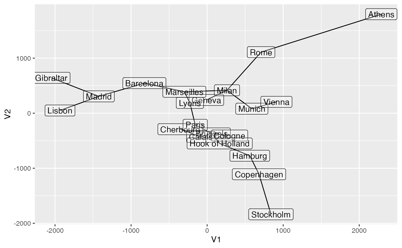
eurodist %>%
cmdscale(k = 6) %>%
as.data.frame() %>%
tibble::rownames_to_column(var = "city") ->
euro_mds
ggplot(euro_mds, aes(V1, V2, label = city)) +
stat_spantree() +
geom_label(alpha = .25)
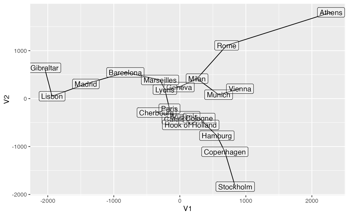 ggplot(euro_mds, aes_c(aes_coord(euro_mds, "V"), aes(label = city))) +
stat_spantree() +
geom_label(aes(x = V1, y = V2), alpha = .25)
ggplot(euro_mds, aes_c(aes_coord(euro_mds, "V"), aes(label = city))) +
stat_spantree() +
geom_label(aes(x = V1, y = V2), alpha = .25)