Project rows onto columns or vice-versa

Compute projections of vectors from one matrix factor onto those of the other.

Usage

stat_projection(
  mapping = NULL,
  data = NULL,
  geom = "segment",
  position = "identity",
  referent = NULL,
  ...,
  show.legend = NA,
  inherit.aes = TRUE
)

Arguments

mapping

Set of aesthetic mappings created by aes(). If specified and inherit.aes = TRUE (the default), it is combined with the default mapping at the top level of the plot. You must supply mapping if there is no plot mapping.

data

The data to be displayed in this layer. There are three options:

If NULL, the default, the data is inherited from the plot data as specified in the call to ggplot().

A data.frame, or other object, will override the plot data. All objects will be fortified to produce a data frame. See fortify() for which variables will be created.

A function will be called with a single argument, the plot data. The return value must be a data.frame, and will be used as the layer data. A function can be created from a formula (e.g. ~ head(.x, 10)).

geom

The geometric object to use to display the data for this layer. When using a stat_*() function to construct a layer, the geom argument can be used to override the default coupling between stats and geoms. The geom argument accepts the following:

A Geom ggproto subclass, for example GeomPoint.
A string naming the geom. To give the geom as a string, strip the function name of the geom_ prefix. For example, to use geom_point(), give the geom as "point".
For more information and other ways to specify the geom, see the layer geom documentation.

position

A position adjustment to use on the data for this layer. This can be used in various ways, including to prevent overplotting and improving the display. The position argument accepts the following:

The result of calling a position function, such as position_jitter(). This method allows for passing extra arguments to the position.
A string naming the position adjustment. To give the position as a string, strip the function name of the position_ prefix. For example, to use position_jitter(), give the position as "jitter".
For more information and other ways to specify the position, see the layer position documentation.

referent

The reference data set; see Details.

...

Additional arguments passed to ggplot2::layer().

show.legend

logical. Should this layer be included in the legends? NA, the default, includes if any aesthetics are mapped. FALSE never includes, and TRUE always includes. It can also be a named logical vector to finely select the aesthetics to display.

inherit.aes

If FALSE, overrides the default aesthetics, rather than combining with them. This is most useful for helper functions that define both data and aesthetics and shouldn't inherit behaviour from the default plot specification, e.g. borders().

Value

A ggproto layer.

Details

An ordination model of continuous data can be used to predict values along one dimension from those along the other, using the artificial axes as intermediaries. The predictions correspond geometrically to projections of elements of one matrix factor in principal coordinates onto those of the other factor in standard coordinates. In the most familiar setting of PCA biplots, variable (column) values are predicted from case (row) locations along PC1 and PC2. This transformation obtains the axis projections as xend,yend and pairs them with original points x,y to demarcate segments visualizing the projections.

WARNING: This layer is appropriate only with axes in standard coordinates (usually confer_inertia(p = "rows")) and predictive calibration (ggbiplot(axis.type = "predictive")).

Referential stats

This statistical transformation is done with respect to reference data passed to referent (ignored if NULL, the default, possibly resulting in empty output). See stat_referent() for more details. This relies on a sleight of hand through a new undocumented LayerRef class and associated ggplot2::ggplot_add() method. As a result, only layers constructed using this stat_*() shortcut will pass the necessary positional aesthetics to the $setup_params() step, making them available to pre-process referent data.

The biplot shortcuts automatically substitute the complementary matrix factor for referent = NULL and will use an integer vector to select a subset from this factor. These uses do not require the mapping passage.

Biplot layers

ggbiplot() uses ggplot2::fortify() internally to produce a single data frame with a .matrix column distinguishing the subjects ("rows") and variables ("cols"). The stat layers stat_rows() and stat_cols() simply filter the data frame to one of these two.

The geom layers geom_rows_*() and geom_cols_*() call the corresponding stat in order to render plot elements for the corresponding factor matrix. geom_dims_*() selects a default matrix based on common practice, e.g. points for rows and arrows for columns.

Ordination aesthetics

This statistical transformation is compatible with the convenience function ord_aes().

Some transformations (e.g. stat_center()) commute with projection to the lower (1 or 2)-dimensional biplot space. If they detect aesthetics of the form ..coord[0-9]+, then ..coord1 and ..coord2 are converted to x and y while any remaining are ignored.

Other transformations (e.g. stat_spantree()) yield different results in a lower-dimensional biplot when they are computed before versus after projection. If the stat layer detects these aesthetics, then the transformation is performed before projection, and the results in the first two dimensions are returned as x and y.

A small number of transformations (stat_rule()) are incompatible with ordination aesthetics but will accept ord_aes() without warning.

Computed variables

These are calculated during the statistical transformation and can be accessed with delayed evaluation.

xend,yend: projections onto (specified) vectors

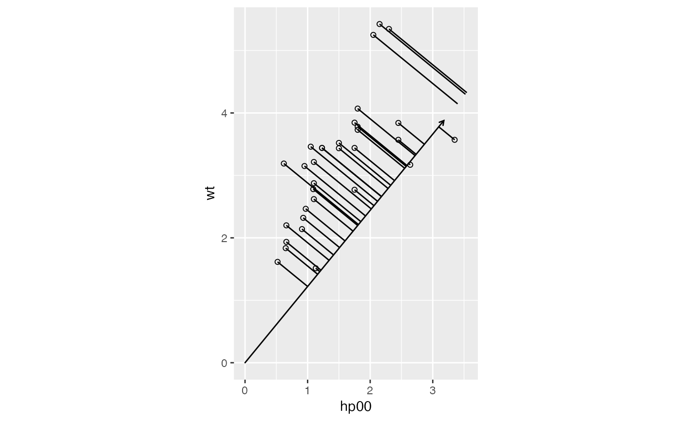
Examples

# simplify the Motor Trends data to two predictors legible at aspect ratio 1
mtcars |>
  transform(hp00 = hp/100) |>
  subset(select = c(mpg, hp00, wt)) ->
  subcars
# compute the gradient of `mpg` against these two predictors
lm(mpg ~ hp00 + wt, subcars) |>
  coefficients() |>
  as.list() |> as.data.frame() ->
  grad
# project the data onto the gradient axis (with a reversed gradient vector)
ggplot(subcars, aes(x = hp00, y = wt)) +
  coord_equal() +
  geom_point(shape = "circle open") +
  geom_vector(data = -grad) +
  stat_projection(referent = grad)