Compute statistics with respect to a reference data set with shared positional variables.
Usage
stat_referent(
  mapping = NULL,
  data = NULL,
  geom = "blank",
  position = "identity",
  referent = NULL,
  show.legend = NA,
  inherit.aes = TRUE,
  ...
)

# S3 method for class 'LayerRef'
ggplot_add(object, plot, ...)
Arguments
- mapping
Set of aesthetic mappings created by
aes(). If specified andinherit.aes = TRUE(the default), it is combined with the default mapping at the top level of the plot. You must supplymappingif there is no plot mapping.- data
The data to be displayed in this layer. There are three options:
If
NULL, the default, the data is inherited from the plot data as specified in the call toggplot().A
data.frame, or other object, will override the plot data. All objects will be fortified to produce a data frame. Seefortify()for which variables will be created.A
functionwill be called with a single argument, the plot data. The return value must be adata.frame, and will be used as the layer data. Afunctioncan be created from aformula(e.g.~ head(.x, 10)).- geom
The geometric object to use to display the data for this layer. When using a
stat_*()function to construct a layer, thegeomargument can be used to override the default coupling between stats and geoms. Thegeomargument accepts the following:A
Geomggproto subclass, for exampleGeomPoint.A string naming the geom. To give the geom as a string, strip the function name of the
geom_prefix. For example, to usegeom_point(), give the geom as"point".For more information and other ways to specify the geom, see the layer geom documentation.
- position
A position adjustment to use on the data for this layer. This can be used in various ways, including to prevent overplotting and improving the display. The
positionargument accepts the following:The result of calling a position function, such as
position_jitter(). This method allows for passing extra arguments to the position.A string naming the position adjustment. To give the position as a string, strip the function name of the
position_prefix. For example, to useposition_jitter(), give the position as"jitter".For more information and other ways to specify the position, see the layer position documentation.
- referent
The reference data set, admitting the same 3 options as
data; see Details.- show.legend
logical. Should this layer be included in the legends?
NA, the default, includes if any aesthetics are mapped.FALSEnever includes, andTRUEalways includes. It can also be a named logical vector to finely select the aesthetics to display. To include legend keys for all levels, even when no data exists, useTRUE. IfNA, all levels are shown in legend, but unobserved levels are omitted.- inherit.aes
If
FALSE, overrides the default aesthetics, rather than combining with them. This is most useful for helper functions that define both data and aesthetics and shouldn't inherit behaviour from the default plot specification, e.g.annotation_borders().- ...
Additional arguments passed to
ggplot2::layer().- object
An object to add to the plot
- plot
The ggplot object to add
objectto
Details
Often in geometric data analysis a statistical transformation applied to data
\(X\) will also depend on data \(Y\), for example when drawing the
projections of vectors \(X\) onto vectors \(Y\). The stat layer
stat_referent() accepts \(Y\) as an argument to the referent argument
and pre-processes them using the existing positional aesthetic mappings to
x and y.
If a function is passed to referent, then the reference data are obtained
by evaluating the function at the primary data. Alongside borrowing the
aesthetic mappings, the evaluation is done during addition via
ggplot2::ggplot_add() of the layer of custom class LayerRef.
The ggproto can be used as a parent to more elaborate statistical
transformations, or the stat can be paired with geoms that expect the
referent argument and use it to position their transformations of \(X\).
It pairs by default to ggplot2::geom_blank() so as to prevent possibly
confusing output.
Examples
# simplify the Motor Trends data to two predictors legible at aspect ratio 1
mtcars %>%
transform(hp00 = hp/100) %>%
subset(select = c(mpg, hp00, wt)) ->
subcars
# compute the gradient of `mpg` against these two predictors
lm(mpg ~ hp00 + wt, subcars) %>%
coefficients() %>%
as.list() %>% as.data.frame() ->
grad
# use the gradient as a reference (to no effect in this basic ggproto)
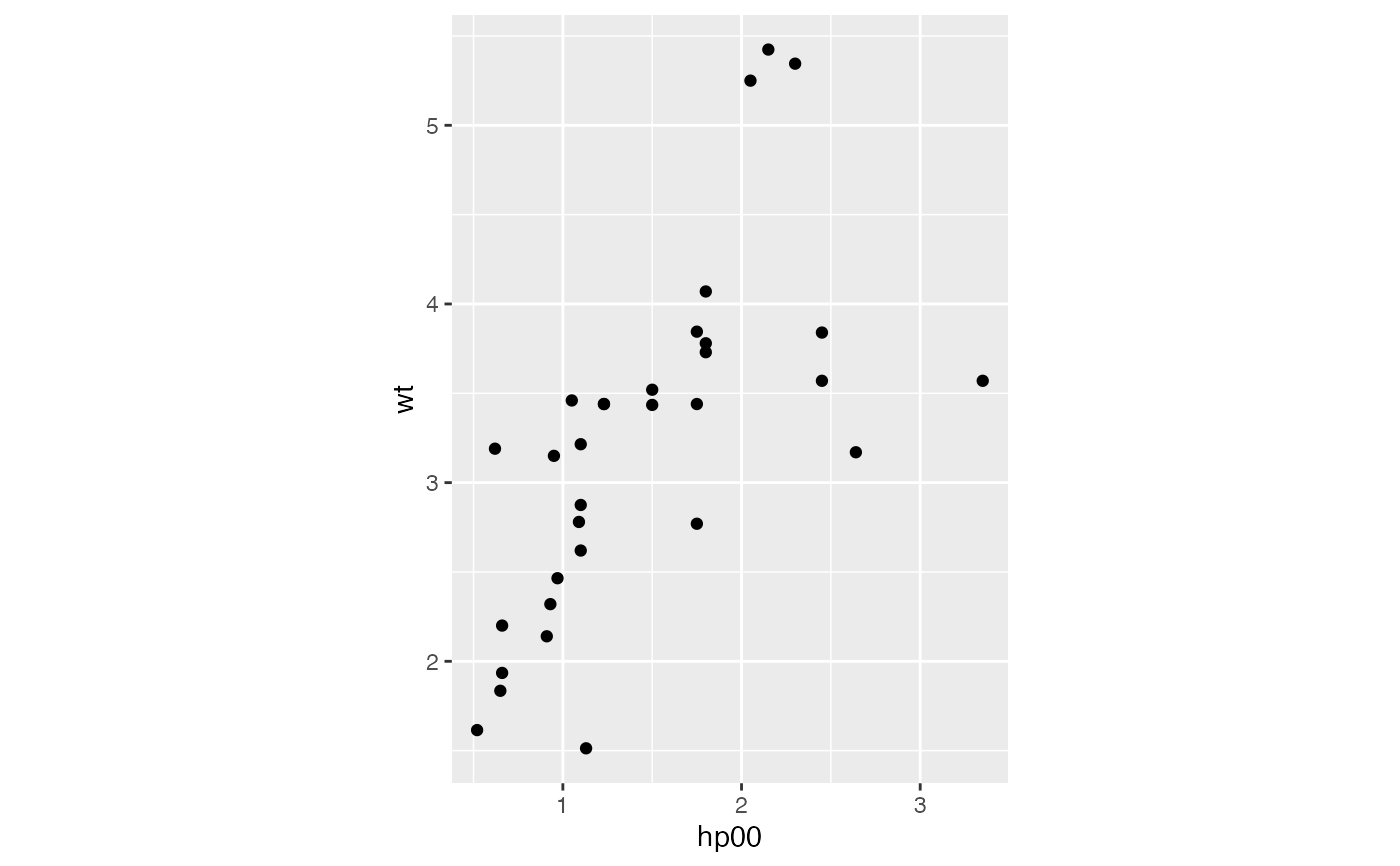
ggplot(subcars, aes(x = hp00, y = wt)) +
coord_equal() +
geom_point() +
stat_referent(referent = grad)
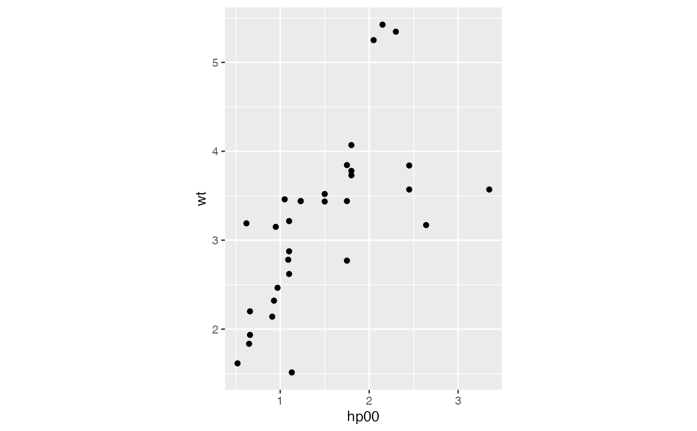
 ggplot(subcars, aes(x = hp00, y = wt)) +
coord_equal() +
stat_referent(geom = "point", referent = grad)
ggplot(subcars, aes(x = hp00, y = wt)) +
coord_equal() +
stat_referent(geom = "point", referent = grad)
 # passing a function yields a transformation of the primary data
p <- ggplot(subcars, aes(x = hp00, y = wt)) +
stat_referent(
data = head,
referent = function(d) as.data.frame(lapply(d, mean))
)
b <- ggplot_build(p)
# original data
b[["plot"]][["data"]]
#> mpg hp00 wt
#> Mazda RX4 21.0 1.10 2.620
#> Mazda RX4 Wag 21.0 1.10 2.875
#> Datsun 710 22.8 0.93 2.320
#> Hornet 4 Drive 21.4 1.10 3.215
#> Hornet Sportabout 18.7 1.75 3.440
#> Valiant 18.1 1.05 3.460
#> Duster 360 14.3 2.45 3.570
#> Merc 240D 24.4 0.62 3.190
#> Merc 230 22.8 0.95 3.150
#> Merc 280 19.2 1.23 3.440
#> Merc 280C 17.8 1.23 3.440
#> Merc 450SE 16.4 1.80 4.070
#> Merc 450SL 17.3 1.80 3.730
#> Merc 450SLC 15.2 1.80 3.780
#> Cadillac Fleetwood 10.4 2.05 5.250
#> Lincoln Continental 10.4 2.15 5.424
#> Chrysler Imperial 14.7 2.30 5.345
#> Fiat 128 32.4 0.66 2.200
#> Honda Civic 30.4 0.52 1.615
#> Toyota Corolla 33.9 0.65 1.835
#> Toyota Corona 21.5 0.97 2.465
#> Dodge Challenger 15.5 1.50 3.520
#> AMC Javelin 15.2 1.50 3.435
#> Camaro Z28 13.3 2.45 3.840
#> Pontiac Firebird 19.2 1.75 3.845
#> Fiat X1-9 27.3 0.66 1.935
#> Porsche 914-2 26.0 0.91 2.140
#> Lotus Europa 30.4 1.13 1.513
#> Ford Pantera L 15.8 2.64 3.170
#> Ferrari Dino 19.7 1.75 2.770
#> Maserati Bora 15.0 3.35 3.570
#> Volvo 142E 21.4 1.09 2.780
# head of original data
b[["data"]][[1]]
#> x y PANEL group
#> 1 1.10 2.620 1 -1
#> 2 1.10 2.875 1 -1
#> 3 0.93 2.320 1 -1
#> 4 1.10 3.215 1 -1
#> 5 1.75 3.440 1 -1
#> 6 1.05 3.460 1 -1
# means of original data
b[["plot"]][["layers"]]$stat_referent$stat_params$referent
#> mpg hp00 wt
#> 1 20.09062 1.466875 3.21725
# means of head of original data
as.data.frame(lapply(layer_data(p, 1), mean))
#> Warning: argument is not numeric or logical: returning NA
#> x y PANEL group
#> 1 1.171667 2.988333 NA -1
# passing a function yields a transformation of the primary data
p <- ggplot(subcars, aes(x = hp00, y = wt)) +
stat_referent(
data = head,
referent = function(d) as.data.frame(lapply(d, mean))
)
b <- ggplot_build(p)
# original data
b[["plot"]][["data"]]
#> mpg hp00 wt
#> Mazda RX4 21.0 1.10 2.620
#> Mazda RX4 Wag 21.0 1.10 2.875
#> Datsun 710 22.8 0.93 2.320
#> Hornet 4 Drive 21.4 1.10 3.215
#> Hornet Sportabout 18.7 1.75 3.440
#> Valiant 18.1 1.05 3.460
#> Duster 360 14.3 2.45 3.570
#> Merc 240D 24.4 0.62 3.190
#> Merc 230 22.8 0.95 3.150
#> Merc 280 19.2 1.23 3.440
#> Merc 280C 17.8 1.23 3.440
#> Merc 450SE 16.4 1.80 4.070
#> Merc 450SL 17.3 1.80 3.730
#> Merc 450SLC 15.2 1.80 3.780
#> Cadillac Fleetwood 10.4 2.05 5.250
#> Lincoln Continental 10.4 2.15 5.424
#> Chrysler Imperial 14.7 2.30 5.345
#> Fiat 128 32.4 0.66 2.200
#> Honda Civic 30.4 0.52 1.615
#> Toyota Corolla 33.9 0.65 1.835
#> Toyota Corona 21.5 0.97 2.465
#> Dodge Challenger 15.5 1.50 3.520
#> AMC Javelin 15.2 1.50 3.435
#> Camaro Z28 13.3 2.45 3.840
#> Pontiac Firebird 19.2 1.75 3.845
#> Fiat X1-9 27.3 0.66 1.935
#> Porsche 914-2 26.0 0.91 2.140
#> Lotus Europa 30.4 1.13 1.513
#> Ford Pantera L 15.8 2.64 3.170
#> Ferrari Dino 19.7 1.75 2.770
#> Maserati Bora 15.0 3.35 3.570
#> Volvo 142E 21.4 1.09 2.780
# head of original data
b[["data"]][[1]]
#> x y PANEL group
#> 1 1.10 2.620 1 -1
#> 2 1.10 2.875 1 -1
#> 3 0.93 2.320 1 -1
#> 4 1.10 3.215 1 -1
#> 5 1.75 3.440 1 -1
#> 6 1.05 3.460 1 -1
# means of original data
b[["plot"]][["layers"]]$stat_referent$stat_params$referent
#> mpg hp00 wt
#> 1 20.09062 1.466875 3.21725
# means of head of original data
as.data.frame(lapply(layer_data(p, 1), mean))
#> Warning: argument is not numeric or logical: returning NA
#> x y PANEL group
#> 1 1.171667 2.988333 NA -1