Compute normal confidence ellipses for ordination factors

These ordination stats are adapted from ggplot2::stat_ellipse().

stat_rows_ellipse(
  mapping = NULL,
  data = NULL,
  geom = "path",
  position = "identity",
  show.legend = NA,
  inherit.aes = TRUE,
  ...,
  type = "t",
  level = 0.95,
  segments = 51
)

stat_cols_ellipse(
  mapping = NULL,
  data = NULL,
  geom = "path",
  position = "identity",
  show.legend = NA,
  inherit.aes = TRUE,
  ...,
  type = "t",
  level = 0.95,
  segments = 51
)

Arguments

mapping	Set of aesthetic mappings created by aes() or aes_(). If specified and inherit.aes = TRUE (the default), it is combined with the default mapping at the top level of the plot. You must supply mapping if there is no plot mapping.
data	The data to be displayed in this layer. There are three options: If NULL, the default, the data is inherited from the plot data as specified in the call to ggplot(). A data.frame, or other object, will override the plot data. All objects will be fortified to produce a data frame. See fortify() for which variables will be created. A function will be called with a single argument, the plot data. The return value must be a data.frame, and will be used as the layer data. A function can be created from a formula (e.g. ~ head(.x, 10)).
geom	The geometric object to use display the data
position	Position adjustment, either as a string, or the result of a call to a position adjustment function.
show.legend	logical. Should this layer be included in the legends? NA, the default, includes if any aesthetics are mapped. FALSE never includes, and TRUE always includes. It can also be a named logical vector to finely select the aesthetics to display.
inherit.aes	If FALSE, overrides the default aesthetics, rather than combining with them. This is most useful for helper functions that define both data and aesthetics and shouldn't inherit behaviour from the default plot specification, e.g. borders().
...	Additional arguments passed to ggplot2::layer().
type	The type of ellipse. The default "t" assumes a multivariate t-distribution, and "norm" assumes a multivariate normal distribution. "euclid" draws a circle with the radius equal to level, representing the euclidean distance from the center. This ellipse probably won't appear circular unless coord_fixed() is applied.
level	The level at which to draw an ellipse, or, if type="euclid", the radius of the circle to be drawn.
segments	The number of segments to be used in drawing the ellipse.

Format

An object of class StatRowsEllipse (inherits from StatEllipse, Stat, ggproto, gg) of length 2.

An object of class StatColsEllipse (inherits from StatEllipse, Stat, ggproto, gg) of length 2.

Biplot layers

ggbiplot() uses ggplot2::fortify() internally to produce a single data frame with a .matrix column distinguishing the subjects ("rows") and variables ("cols"). The stat layers stat_rows() and stat_cols() simply filter the data frame to one of these two.

The geom layers geom_rows_*() and geom_cols_*() call the corresponding stat in order to render plot elements for the corresponding factor matrix. geom_dims_*() selects a default matrix based on common practice, e.g. points for rows and arrows for columns.

Examples

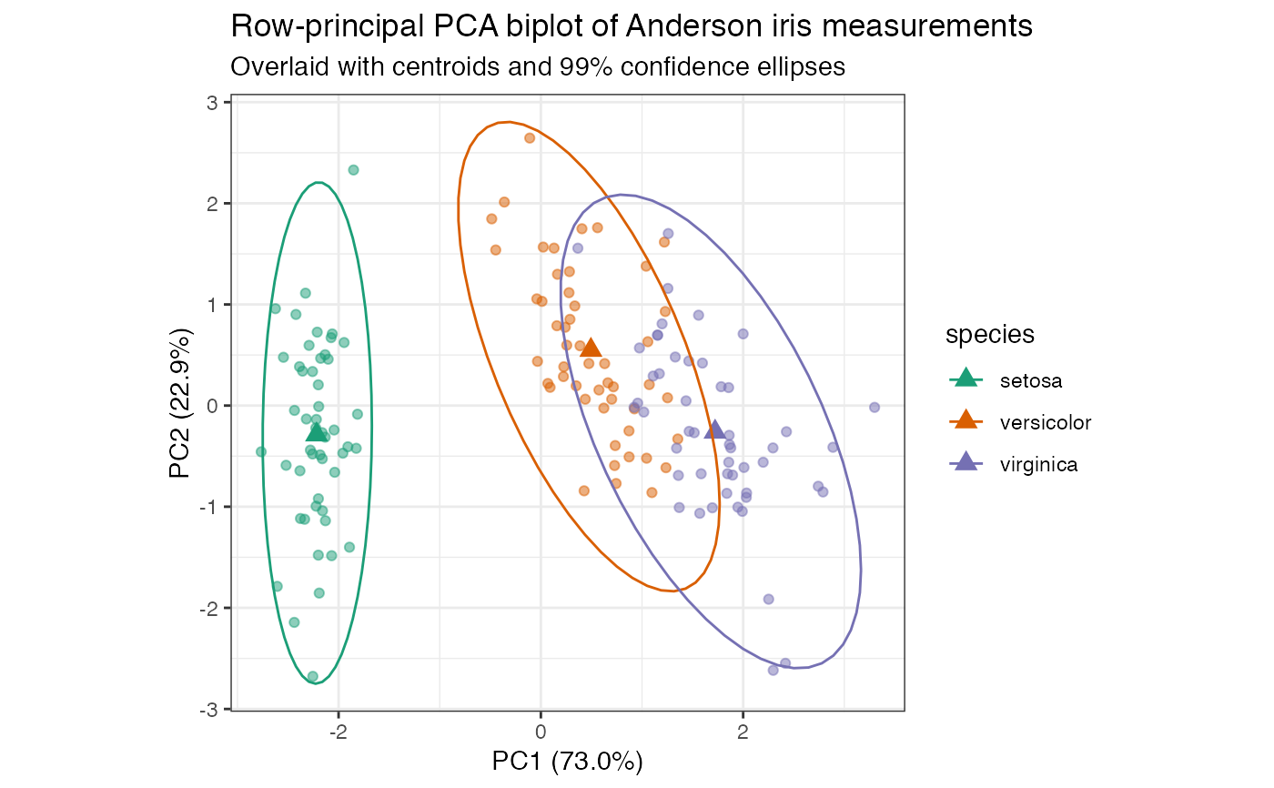
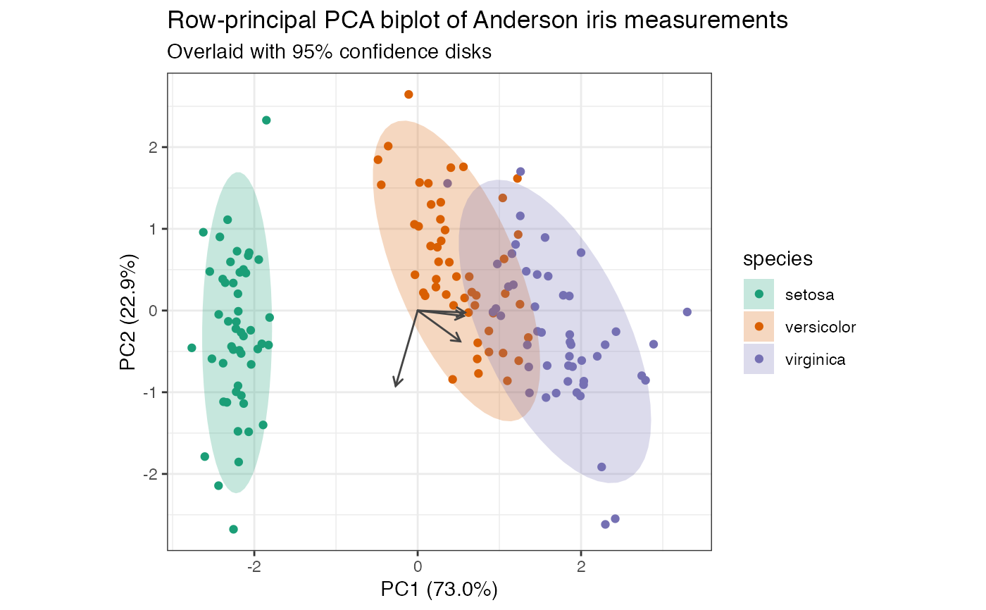
# compute row-principal components of scaled iris measurements
iris[, -5] %>%
  prcomp(scale = TRUE) %>%
  as_tbl_ord() %>%
  mutate_rows(species = iris$Species) %>%
  print() -> iris_pca
#> # A tbl_ord of class 'prcomp': (150 x 4) x (4 x 4)'
#> # 4 coordinates: PC1, PC2, ..., PC4
#> # 
#> # Rows: [ 150 x 4 | 1 ]
#>     PC1    PC2     PC3 ... |   species
#>                            |   <fct>  
#> 1 -2.26 -0.478  0.127      | 1 setosa 
#> 2 -2.07  0.672  0.234  ... | 2 setosa 
#> 3 -2.36  0.341 -0.0441     | 3 setosa 
#> 4 -2.29  0.595 -0.0910     | 4 setosa 
#> 5 -2.38 -0.645 -0.0157     | 5 setosa 
#> # … with 145 more rows
#> # 
#> # Columns: [ 4 x 4 | 0 ]
#>      PC1     PC2    PC3 ... | 
#>                             | 
#> 1  0.521 -0.377   0.720     | 
#> 2 -0.269 -0.923  -0.244 ... | 
#> 3  0.580 -0.0245 -0.142     | 
#> 4  0.565 -0.0669 -0.634     | 
# row-principal biplot with centroids and confidence ellipses
iris_pca %>%
  ggbiplot(aes(color = species)) +
  theme_bw() +
  scale_color_brewer(type = "qual", palette = 2) +
  geom_rows_point(alpha = .5) +
  stat_rows_center(fun.center = "mean", size = 3, shape = "triangle") +
  stat_rows_ellipse(level = .99) +
  ggtitle(
    "Row-principal PCA biplot of Anderson iris measurements",
    "Overlaid with centroids and 99% confidence ellipses"
  )
# row-principal biplot with centroids and confidence elliptical disks
iris_pca %>%
  ggbiplot(aes(color = species)) +
  theme_bw() +
  geom_rows_point() +
  geom_polygon(
    aes(fill = species),
    color = NA, alpha = .25, stat = "rows_ellipse"
  ) +
  geom_cols_vector(color = "#444444") +
  scale_color_brewer(
    type = "qual", palette = 2,
    aesthetics = c("color", "fill")
  ) +
  ggtitle(
    "Row-principal PCA biplot of Anderson iris measurements",
    "Overlaid with 95% confidence disks"
  )