Analysis of a Toy Example • plt

This vignette reproduces the analysis of a toy example in Sections 5.2–5.7 of Bubenik and Dłotko (2017).¹

library(plt)

The purpose of this example is to illustrate the Persistence Landscapes Toolbox for summarizing and discriminating among point cloud data based on their persistent homology. The toy data comprise several point clouds sampled from unions of pairwise tangent unit circles; see the example after the sampler below (c.f. Section 5.2):

# sample `50 * n` points from `n` concatenated circles with uniform noise
sample_tangent_circles <- function(n) {
  # bind rows from several samples
  do.call(rbind, lapply(seq(0L, n - 1L), function(m) {
    # sample from the unit circle
    tdaunif::sample_circle(n = 50L) +
      # shift this circle `m` units rightward
      matrix(rep(c(2 * m, 0), each = 50L), ncol = 2L) +
      # add uniform noise
      matrix(runif(n = 50L * 2L, min = -0.15, max = 0.15), ncol = 2L)
  }))
}
# illustrate with a 5-circle sequence
plot(sample_tangent_circles(n = 5L), pch = "+", col = "red", asp = 1)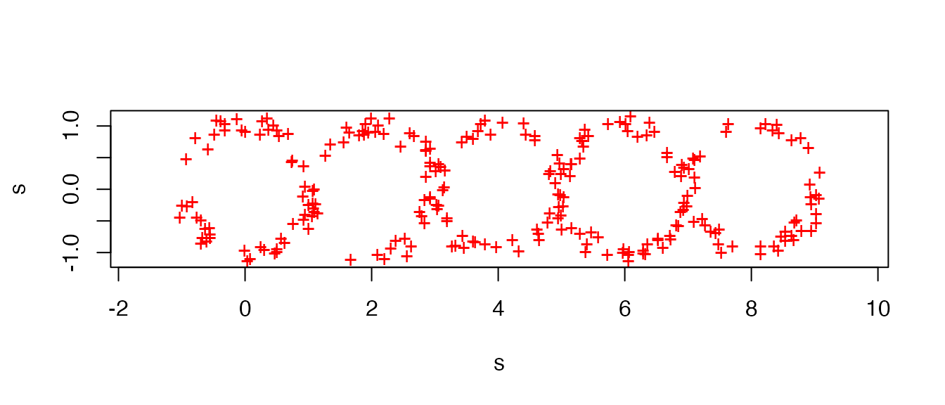

Here we generate all $5 * 11 = 55$ samples and store their degree-1 persistence landscapes. We include a scale factor that recovers landscapes at the same scale as those reported in the paper:

# define scale factor
sf <- 55
# initialize list
toy_pl <- vector("list", 5L)
# populate each position in the list
for (n in seq_along(toy_pl)) {
  # initialize sub-list
  toy_n <- vector("list", 11L)
  # draw 11 samples
  for (i in seq(11L)) {
    toy_data <- sample_tangent_circles(n)
    # scale data by scale factor
    toy_data[, ] <- toy_data[, ] * sf
    # calculate persistent homology, up to the diameter of the subspace
    ph <- suppressWarnings(
      ripserr::vietoris_rips(toy_data, dim = 1, threshold = n * 2 * sf)
    )
    # format as persistence data
    pd <- as_persistence(ph)
    # construct degree-1 persistence landscape
    pl <- pl_new(pd, degree = 1L, exact = TRUE)
    # store the landscape
    toy_n[[i]] <- pl
  }
  toy_pl[[n]] <- toy_n
}

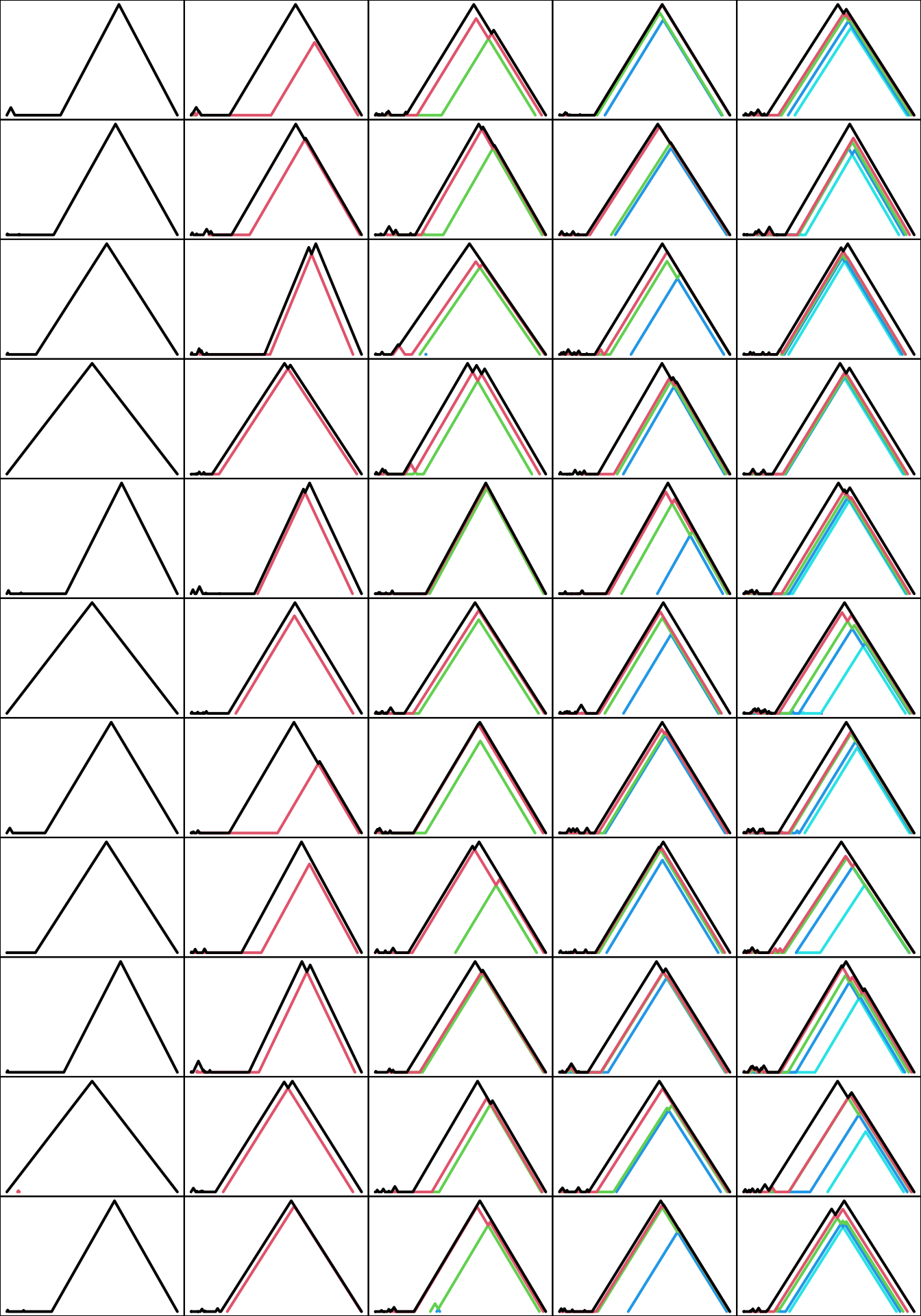
Each landscape contains as many significant levels as circles made up the sample space. In the plots below, tick marks are omitted to make more space for the landscapes themselves:

par(mfcol = c(11L, 5L), mar = c(0, 0, 0, 0))
for (n in seq_along(toy_pl)) for (i in seq_along(toy_pl[[n]])) {
  plot(toy_pl[[n]][[i]], xaxt = "n", yaxt = "n")
}

The commonalities of the samples from each space can be revealed by taking their mean landscapes (c.f. Section 5.4):

# calculate means
toy_pl_mean <- lapply(toy_pl, pl_mean)
# plot  means
par(mfcol = c(1L, 5L), mar = c(0, 0, 0, 0))
for (n in seq_along(toy_pl_mean)) {
  plot(toy_pl_mean[[n]], xaxt = "n", yaxt = "n")
}

Below we compute the $1$ -, $2$ -, and $\infty$ -norms of these mean landscapes (c.f. Section 5.5):

# norms to calculate
ps <- c(1, 2, Inf)
# initialize matrix
toy_pl_norms <- matrix(NA_real_, nrow = 5L, ncol = 3L)
rownames(toy_pl_norms) <- paste0(seq(5L), "-circle")
colnames(toy_pl_norms) <- paste0("p = ", ps)
# populate matrix
for (n in seq_along(toy_pl_mean)) for (p in seq_along(ps)) {
  # calculate norm
  toy_pl_norms[n, p] <- pl_norm(toy_pl_mean[[n]], ps[[p]])
}
# print matrix
print(toy_pl_norms)
#>              p = 1    p = 2  p = Inf
#> 1-circle  777.3095 118.5246 26.02017
#> 2-circle 1783.4118 185.7788 29.48225
#> 3-circle 2430.9508 210.5853 29.24994
#> 4-circle 3343.0838 251.6085 31.01226
#> 5-circle 4081.0200 277.3163 30.87295

Below we compute the pairwise $2$ -distances between the mean landscapes (c.f. Section 5.6):

# compute distance matrix
pl_dist(toy_pl_mean)
#>          [,1]      [,2]      [,3]      [,4]      [,5]
#> [1,]   0.0000 121.66729 156.72068 205.81555 235.31593
#> [2,] 121.6673   0.00000  95.45027 150.94825 187.10785
#> [3,] 156.7207  95.45027   0.00000  95.81676 143.13606
#> [4,] 205.8155 150.94825  95.81676   0.00000  88.71722
#> [5,] 235.3159 187.10785 143.13606  88.71722   0.00000

Section 5.7 reports that permutation tests between the sample landscapes from different numbers $n$ of circles all obtained p-values near zero, successfully detecting the differences between the samples. Below we report two permutation tests, between the samples $n=1$ and $n=2$ and between the samples $n=4$ and $n=5$ :

# compare 1-circle and 2-circle samples
pl_perm_test(toy_pl[[1L]], toy_pl[[2L]])
#> 
#>  permutation test
#> 
#> data:  
#> p-value < 2.2e-16
#> alternative hypothesis: true distance between mean landscapes is greater than 0
#> sample estimates:
#> distance between mean landscapes 
#>                         121.6673
# compare 4-circle and 5-circle samples
pl_perm_test(toy_pl[[4L]], toy_pl[[5L]])
#> 
#>  permutation test
#> 
#> data:  
#> p-value < 2.2e-16
#> alternative hypothesis: true distance between mean landscapes is greater than 0
#> sample estimates:
#> distance between mean landscapes 
#>                         88.71722

To test the specificity, rather than the sensitivity, of the permutation test, below we generate additional, smaller samples from the 1- and 5-circle spaces and perform permutation tests between them and their original counterparts from the same spaces:

# draw a new 1-circle sample
new_pl_1 <- vector("list", 6L)
for (i in seq(6L)) {
  toy_data <- sample_tangent_circles(1)
  toy_data[, ] <- toy_data[, ] * sf
  ph <- suppressWarnings(
    ripserr::vietoris_rips(toy_data, dim = 1, threshold = 1 * 2 * sf)
  )
  pd <- as_persistence(ph)
  pl <- pl_new(pd, degree = 1L, exact = TRUE)
  new_pl_1[[i]] <- pl
}
# compare old & new 1-circle samples
pl_perm_test(toy_pl[[1L]], new_pl_1)
#> 
#>  permutation test
#> 
#> data:  
#> p-value = 0.389
#> alternative hypothesis: true distance between mean landscapes is greater than 0
#> sample estimates:
#> distance between mean landscapes 
#>                          13.6971

# draw a new 5-circle sample
new_pl_5 <- vector("list", 6L)
for (i in seq(6L)) {
  toy_data <- sample_tangent_circles(5)
  toy_data[, ] <- toy_data[, ] * sf
  ph <- suppressWarnings(
    ripserr::vietoris_rips(toy_data, dim = 1, threshold = 5 * 2 * sf)
  )
  pd <- as_persistence(ph)
  pl <- pl_new(pd, degree = 1L, exact = TRUE)
  new_pl_5[[i]] <- pl
}
# compare old & new 5-circle samples
pl_perm_test(toy_pl[[5L]], new_pl_5)
#> 
#>  permutation test
#> 
#> data:  
#> p-value = 0.454
#> alternative hypothesis: true distance between mean landscapes is greater than 0
#> sample estimates:
#> distance between mean landscapes 
#>                         22.58901

Bubenik P & Dłotko P (2017) “A persistence landscapes toolbox for topological statistics”. Journal of Symbolic Computation 78(1):91–114. https://www.sciencedirect.com/science/article/pii/S0747717116300104 ↩︎