Integrals, Distances, and Norms of Persistence Landscapes

Calculate distances and perform infinitesimal calculus on persistence landscapes. See Section 3 of Bubenik (2015).

pl_integrate(pl, p = 1)

pl_distance(pl1, pl2, p = 2)

pl_dist(pl_list, p = 2)

pl_norm(pl, p = 2)

pl_indicator(pl, supports, r = 0)

pl_indicator_form(pl, supports, r = 0, p = 1)

Arguments

pl

A persistence landscape as returned by pl_new().

p

Positive integer or infinity; the power used to compute an integral.

pl1, pl2

Persistence landscapes.

pl_list

A list of persistence landscapes. A non-list object will first be wrapped in a list.

supports

List of support intervals for landscape levels.

r

Non-negative number; the power of the coefficient \(1/k\) in the indicator linear form.

Value

A persistence landscape (an object of S4 class 'Rcpp_PersistenceLandscape'), a real number, or a vector of real numbers.

Details

pl_integrate() computes the \(L^p\) integral of a persistence landscape. The p parameter denotes the integral's power; p = 1 computes the area under the curves, while p = 2 corresponds to the \(L^2\) norm. Letting p = Inf returns the maximum landscape height.

pl_distance() calculates the \(L^p\) distance between two persistence landscapes.

pl_dist() utilizes pl_distance() to compute all pairwise distances between a list of landscapes. It returns a symmetric matrix of distances.

pl_norm() returns the \(L^p\) norm of a single landscape, used as a scalar summary of its magnitude. Similar to pl_integrate(), it supports all finite powers p >= 1, as well as p = Inf for the supremum norm.

pl_indicator() computes the linear form defined by a sum of indicator functions over user-specified support intervals, weighted by \(1/k^r\) where \(k\) indexes the landscape levels.

pl_indicator_form() evaluates the integral of the indicator function form described above with respect to the \(L^p\) norm. It returns a real number representing the landscape's integral onto the chosen intervals.

See also

arithmetic, algebra, inference for other landscape functions.

Examples

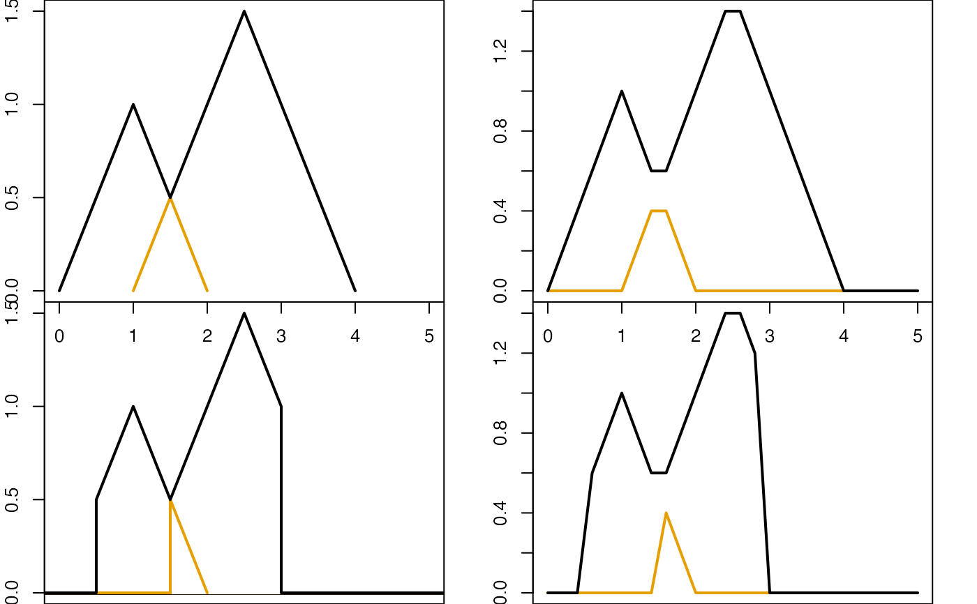
# multiply by an indicator function
pd <- data.frame(dimension = 1, birth = c(0, 1), death = c(2, 4))
f <- list(c(.5, 3), c(1.5, 2), c(1.75, 2))

# exact landscape
pl_e <- pl_new(pd, degree = 1, exact = TRUE)
par(mfcol = c(2L, 2L), mar = c(0, 2, 0, 2))
plot(pl_e, xlim = c(0, 5))
# pl_ef <- pl$indicator(f, 0)
pl_ef <- pl_indicator(pl_e, f)
plot(pl_ef, xlim = c(0, 5))
# discrete landscape
pl_d <- pl_new(pd, degree = 1, xmin = 0, xmax = 5, xby = .2)
plot(pl_d)
# pl_df <- pl_d$indicator(f, 0)
pl_df <- pl_indicator(pl_d, f)
plot(pl_df, xlim = c(0, 5))

par(mfrow = c(1L, 1L), mar = c(5.1, 4.1, 4.1, 2.1))

# integrate PL multiplied by an indicator function
pl_indicator_form(pl_d, supports = f, p = 5)
#> [1] 3.499947
pl_integrate(pl_df, p = 5)
#> [1] 3.499947
pl_indicator_form(pl_e, supports = f, p = 5)
#> [1] 3.958333
pl_integrate(pl_ef, p = 5)
#> [1] 3.958333