Classes for workhorse matrix decompositions

...

eigen_ord(x, symmetric = isSymmetric.matrix(x))

svd_ord(x, nu = min(dim(x)), nv = min(dim(x)))

Arguments

x	a numeric or complex matrix whose spectral decomposition is to be computed. Logical matrices are coerced to numeric.
symmetric	if TRUE, the matrix is assumed to be symmetric (or Hermitian if complex) and only its lower triangle (diagonal included) is used. If symmetric is not specified, isSymmetric(x) is used.
nu	the number of left singular vectors to be computed. This must between 0 and n = nrow(x).
nv	the number of right singular vectors to be computed. This must be between 0 and p = ncol(x).

Examples

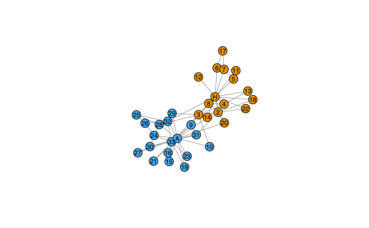
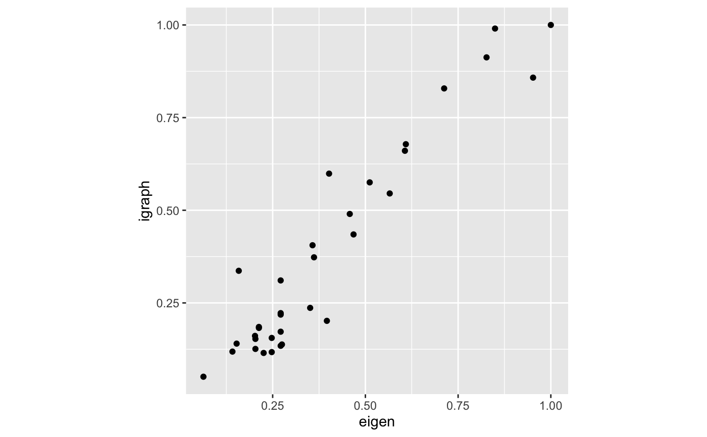
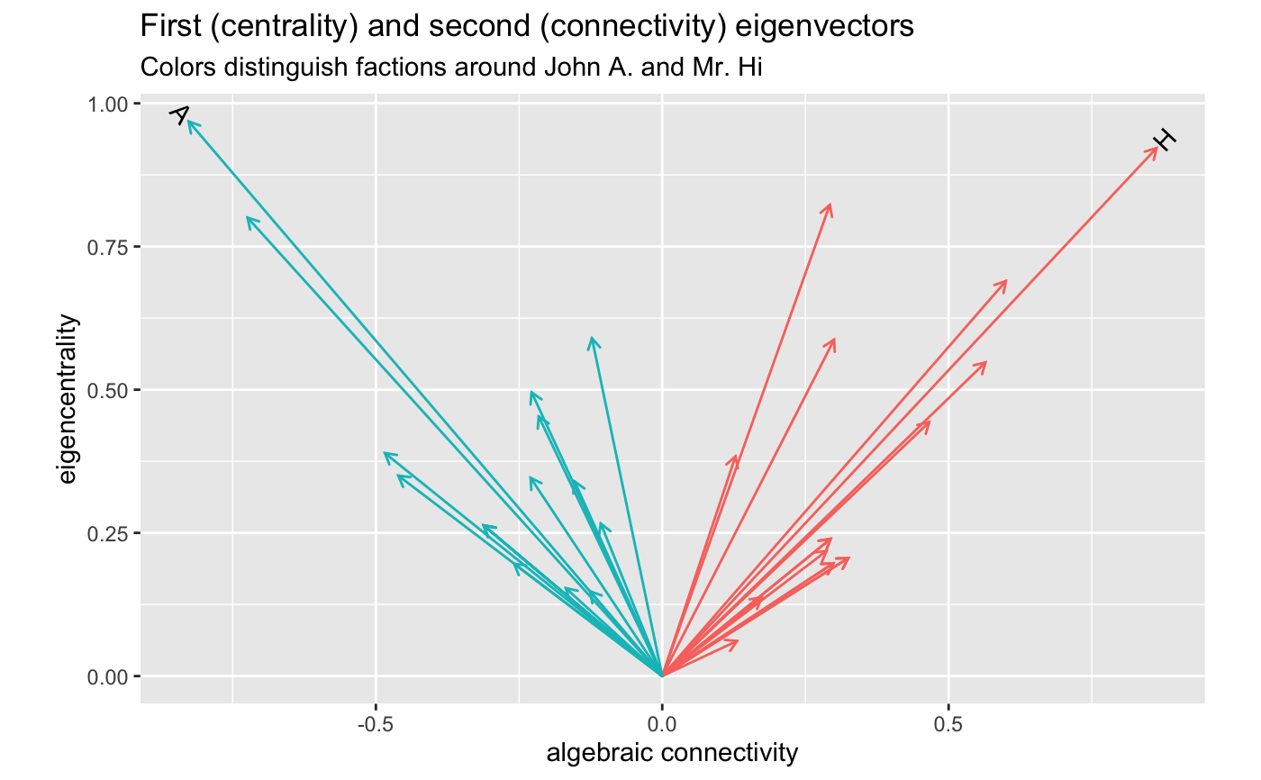
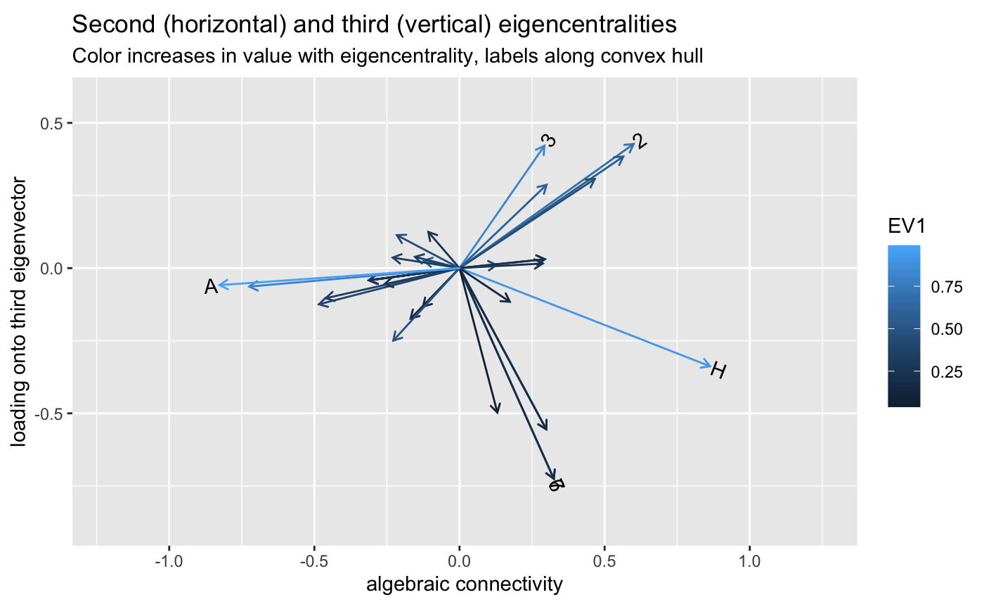
# Graph Laplacian eigenvectors for spectral partitioning
data(karate, package = "igraphdata")
igraph::plot.igraph(
  karate,
  vertex.label.family = "sans",
  vertex.label.color = "black",
  vertex.label.cex = .75
)
# first eigenvector (centrality)
karate_eigen_cent <- igraph::eigen_centrality(karate)
# eigendecomposition
karate %>%
  igraph::as_adjacency_matrix(sparse = FALSE) %>%
  eigen_ord() %>% as_tbl_ord() %>%
  mutate_u(
    faction = igraph::vertex_attr(karate, "Faction"),
    name = igraph::vertex_attr(karate, "name"),
    label = igraph::vertex_attr(karate, "label")
  ) %>%
  print() -> karate_eigen
#> # A tbl_ord of class 'eigen': (34 x 15) x (34 x 15)'
#> # 15 coordinates: EV1, EV2, ..., EV15
#> # 
#> # U: [ 34 x 15 | 3 ]
#>     EV1   EV2    EV3 ... |   faction name    label
#>                          |     <dbl> <chr>   <chr>
#> 1 0.922 0.863 -0.338     | 1       1 Mr Hi   H    
#> 2 0.690 0.600  0.427 ... | 2       1 Actor 2 2    
#> 3 0.823 0.293  0.421     | 3       1 Actor 3 3    
#> 4 0.548 0.564  0.384     | 4       1 Actor 4 4    
#> 5 0.197 0.299 -0.555     | 5       1 Actor 5 5    
#> # … with 29 more rows
#> # 
#> # V: [ 34 x 15 | 0 ]
#>     EV1   EV2    EV3 ... | 
#>                          | 
#> 1 0.922 0.863 -0.338     | 
#> 2 0.690 0.600  0.427 ... | 
#> 3 0.823 0.293  0.421     | 
#> 4 0.548 0.564  0.384     | 
#> 5 0.197 0.299 -0.555     | 
#> 
# corroborate eigencentralities
tibble::tibble(
  igraph = karate_eigen_cent$vector,
  eigen = karate_eigen$vectors[, 1] / max(karate_eigen$vectors[, 1])
) %>%
  ggplot(aes(x = eigen, y = igraph)) +
  coord_equal() +
  geom_point()
# first and second eigenvectors for centrality and connectivity / partitioning
karate_eigen %>%
  ggbiplot(aes(x = 2, y = 1)) +
  geom_u_vector(aes(color = as.factor(faction))) +
  geom_u_text_radiate(aes(label = ifelse(grepl("H|A", label), label, NA))) +
  guides(color = FALSE) +
  labs(x = "algebraic connectivity", y = "eigencentrality") +
  ggtitle(
    "First (centrality) and second (connectivity) eigenvectors",
    "Colors distinguish factions around John A. and Mr. Hi"
  )
#> Warning: Removed 32 rows containing missing values (geom_text_radiate).
# second and third eigenvectors
karate_eigen %>%
  ggbiplot(aes(x = 2, y = 3)) +
  scale_x_continuous(expand = expand_scale(mult = .3)) +
  scale_y_continuous(expand = expand_scale(mult = .2)) +
  geom_u_vector(aes(color = EV1)) +
  geom_u_text_radiate(stat = "chull", aes(label = label)) +
  labs(x = "algebraic connectivity", y = "loading onto third eigenvector") +
  ggtitle(
    "Second (horizontal) and third (vertical) eigencentralities",
    "Color increases in value with eigencentrality, labels along convex hull"
  )