Exploratory and Predictive Analysis

The goal of Topological data analysis (TDA) is to analyze and measure the global topological features of data. The persistence diagram, a common topological summary, lacks key properties to make it conformable for statistical hypothesis testing and machine learning. Persistence landscapes, introduced by Bubenik (2015)¹, are a vectorization of persistence diagrams. In this vignette, we will show how {plt} supports the computation of persistence landscapes, and both exploratory and predictive analysis. This vignette is based on Peter Bubenik’s TDA labs².

Applications of TDA often proceed along the following steps:

Represent a sample of data as a point cloud.
Construct a filtered simplicial complex on the point cloud.
Obtain the persistence module by taking the simplicial homology of the filtration.
Represent the persistence model as a persistence diagram.
Vectorize the persistence diagram to obtain analysis-ready features.
Use the features in hypothesis testing or machine learning.

This vignette will include dimension reduction, two-sample hypothesis testing, and supervised classification as applications of TDA.

Interoperability

{plt} is designed to be used with other TDA packages such as those loaded below.

The {tdaunif} package provides tools to take uniform random samples from simple manifolds and is commonly used for testing TDA tools. The {TDA} package contains various tools for TDA, including functions to compute persistence data from point clouds and distance matrices. We use the alphaComplexDiag() function to obtain the birth and death values of the alpha complex persistence module.

# for manifold samples
library(tdaunif)
# for alpha shapes
library(alphahull)
# for persistent homology
library(TDA)
# for persistence landscapes!
library(plt)
# for support vector machines
library(e1071)

Persistent Homology of Point Clouds

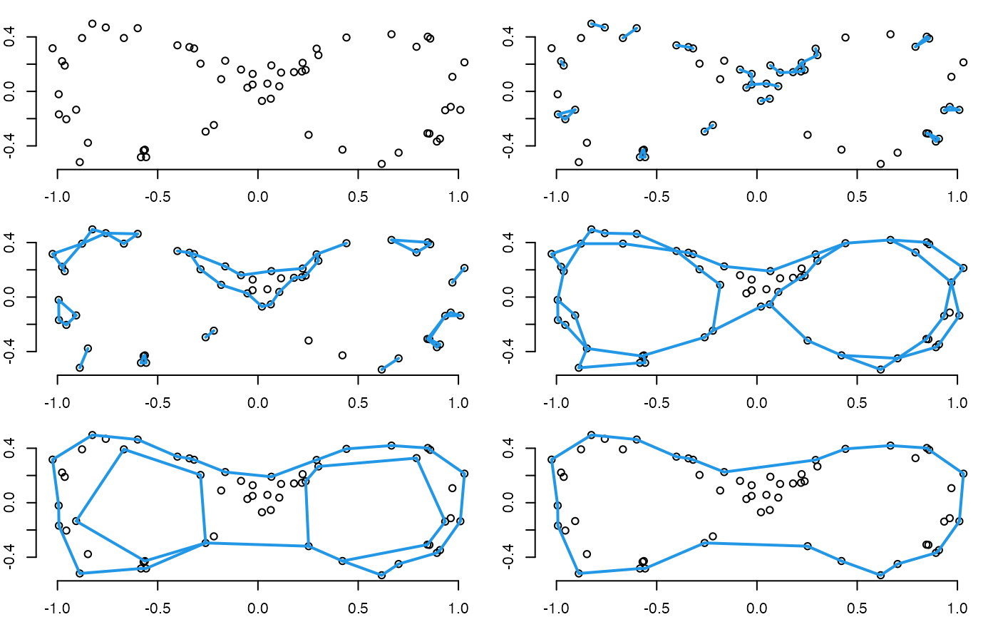
To begin, we create a simple point cloud on which we will illustrate how to use {plt}. We noisily sample $60$ points in $\mathbb{R}^2$ from a figure eight, the lemniscate of Gerono.

set.seed(120246L)
pc <- sample_lemniscate_gerono(n = 60, sd = 0.05)
plot(pc, asp = 1, pch = 16L, main = "Figure Eight Point Cloud")

From our point set, we would like to generate more topologically informative data. We construct a simplicial complex $K$ , which is a set of simplices. A $0$ -simplex is a single point, a $1$ -simplex is an edge or line segment, a $2$ -simplex is a triangle, and a $3$ -simplex is a tetrahedron.

There are different formulations for constructing simplicial complexes that have their own advantages and disadvantages. We will utilize the alpha complex as it captures the underlying structure of the data accurately and is more computationally efficient than other methods.

By applying the alpha complex with various radii (scale), we create a filtered simplicial complex or filtration, which is a nested sequence of simplicial complexes: $K_0 \subset K_1 \subset K_2 \subset \cdots\subset K_n,$ where $n \in \mathbb{N}$ is the number of simplicial complexes in the filtration. For any pair of adjacent terms (simplicial complexes) in the filtration, the preceding term is a subcomplex of the succeeding term.

The plots below illustrate a filtration using alpha shapes (which closely resemble alpha complexes) at six levels of its distance threshold $\epsilon_\alpha$ . As $\epsilon_\alpha$ increases, the number of connected components and loops changes. However, some topological features, such as the two lobes of the figure eight, persist throughout many values of $\epsilon_\alpha$ .

Compute Persistence Data

The filtration provides a mathematical structure for analyzing the global topological features of a point cloud. For each simplicial complex within the filtration, we apply simplicial homology to classify them using Betti numbers. The $k^{\text{th}}$ Betti number $\beta_k$ counts the number of $k$ -dimensional features of a simplicial complex. $\beta_0$ counts the number of $0$ -dimensional connected components, $\beta_1$ counts the number of $1$ -dimensional loops, and $\beta_2$ counts the number of $3$ -dimensional cavities.

Applying simplicial homology to the filtration, we obtain a sequence of vector spaces and linear maps called a persistence module: $H_k(K_0) \rightarrow H_k(K_1) \rightarrow H_k(K_2) \rightarrow \cdots \rightarrow H_k(K_n).$ The persistence module tracks the lifetime of features throughout the time span of the filtration. The birth value $b$ of a feature is when it first appears in the persistence module. The death value $d$ of a feature is when it disappears. A topological feature with a long lifetime $d-b$ is called a persistent feature.

pd <- alphaComplexDiag(pc, maxdimension = 1)$diagram

# birth and death values have been squared, so take the square root
pd[,c(2,3)] <- sqrt(pd[,c(2,3)])

The pd object stores the birth and death values for the $0$ and $1$ dimension features across the alpha filtration.

head(pd)
#>      dimension Birth     Death
#> [1,]         0     0       Inf
#> [2,]         0     0 0.1490153
#> [3,]         0     0 0.1417039
#> [4,]         0     0 0.1220746
#> [5,]         0     0 0.1173572
#> [6,]         0     0 0.1129086

Persistence Diagram

The persistence diagram is a topological summary that visualizes the birth and death times of topological features. The diagram has axes birth & death, and a line $d = b$ . For any point $(b,d)$ , we have $d-b \geq 0$ . Graphically, each point is on or above the $d = b$ line. Points close to or on this line are ephemeral features because they die shortly or immediately after being born.

In the persistence diagram below, three features stand out. Two are $1$ -dimensional features distinguished by their distance from the line $d = b$ . These persistence features represent the two lobes of the figure eight. We also observe a $0$ -dimensional feature with infinite persistence because there must always be the one connected component that includes the entire dataset. As smaller components merge, this final component persists across all scales, since nothing remains to connect with it.

plot(pd, asp = 1, diagLim = c(0,.75))
legend(0.6, 0.4, c('Homology in degree 0','Homology in degree 1'),
col = c(1,2), pch = c(19,2), cex = .8, pt.lwd = 2, bty = "n")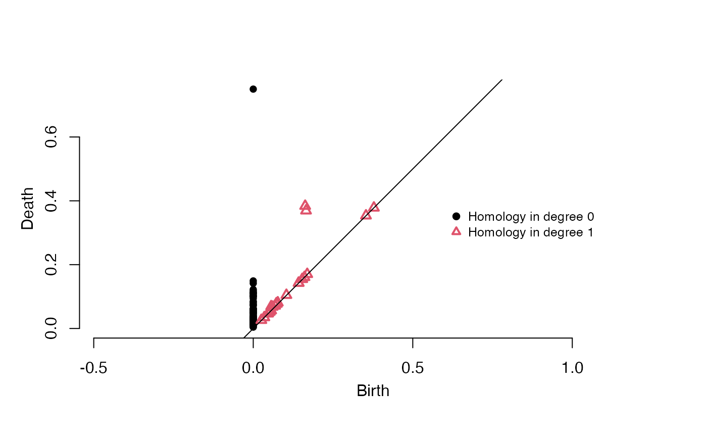

Persistence Landscape Transformation

Now that we have persistence data, we can construct persistence landscapes, which are useful for analyzing topological features in a form suited for statistical methods. Persistence landscapes are built by transforming persistence diagrams into a sequence of “tent” functions that capture the lifetime of topological features.

Tent Functions

Each point in the persistence diagram corresponds to a topological feature with a birth and death time. We can represent these features using tent functions:

The base of the tent spans from the feature’s birth to its death.
The peak of the tent is located at the midpoint between birth and death.
The height of the tent at any point reflects how long the feature persists around that time.

These tent functions are given by: $f_{(b_i, d_i)}(x) = \begin{cases} x - b_i & \text{if } b_i < x \leq \frac{b_i + d_i}{2} \\ -x + d_i & \text{if } \frac{b_i + d_i}{2} < x < d_i \\ 0 & \text{otherwise} \end{cases}$

Levels

To create the persistence landscape, we superimpose these tent functions. At each point on the timeline, the height of the landscape is given by the level of these tents—the largest height at that point. The level provides a layered structure:

$\lambda_1(t)$ is the level that takes the value of the tallest tent at $t$
$\lambda_2(t)$ is the level that takes the value of the second tallest tent at $t$ , and so on for the remaining less prominent features.
Generically, $\lambda_k(t)=k^{\text{th}}$ largest value of $\{f_{(b_i, d_i)}(t) | (b_i, d_i) \in PD\}$ at each $t$ where $PD$ is the persistence diagram. This superimposition of tents, creating a level of functions, allows us to visualize and analyze the relative significance of topological features. The collection of our levels makes our landscape.

These levels help develop a geometric understanding of persistence landscapes and should be helpful for when we think about the analysis being done.

To begin working with the persistence landscape framework, {plt} methods demands that our data is in a particular format, as_persistence() ensures this, if your data is in one of the recognized formats/classes (see help file).

This function in {plt} has multiple methods to convert persistence data to a format required for other {plt} functions. It can be applied to a $3$ -column matrix (or an object coercible to one) with columns dimension/degree, start/birth, and end/death, though the columns need not be named, or it can convert outputs from persistence data producing functions like alphaComplexDiag().

Note that as_persistence() is called in pl_new().

pd <- as_persistence(pd)
print(pd)
#> 'persistence' data computed up to degree 1:
#> 
#> * 0-degree features: 60
#> * 1-degree features: 23
#> 
#> threshold = 0.147231

The pl_new() function takes in a single matrix of persistence data or a formatted list with the class persistence_diagram, and computes the persistence landscape. Below, we compute the landscape for the $1$ -dimensional topological features.

Often users will find it useful to only look at one dimension of the data, whether for simplification or if it’s a particular dimension of interest. Below, we filter for only degree-one topological features and the entire domain of the landscape by setting xmin and xmax to the infimum and supremum, respectively. You can select what window of filtration you want the landscape by changing these parameters. The window must contain the support of the landscape, which is the set of points for which the persistence landscape is non-zero.

pl1d <- pl_new(pd, degree = 1, xby = 0.025)
summary(pl1d)
#> Internal representation:  discrete 
#> Number of levels:  23 
#> Representation limits: ( 0 , 0.4 )  at resolution 0 
#> Landscape range: ( 0 , 0.10871 ) 
#> Magnitude:  0.001612 
#> Integral:   0.022786

The above function for the “tents” performs a transformation that puts each feature in terms of $\frac{b+d}{2}$ and $\frac{d-b}{2}$ , making the graphical representation easier to visually understand. Note that this is a discrete persistence landscape so it is generated by sampling a number of points and interpolating to create a continuous function.

n_levs <- max(pl_num_levels(pl1d))
plot(pl1d, main = "Persistence Landscape", n_levels = n_levs, asp = 1)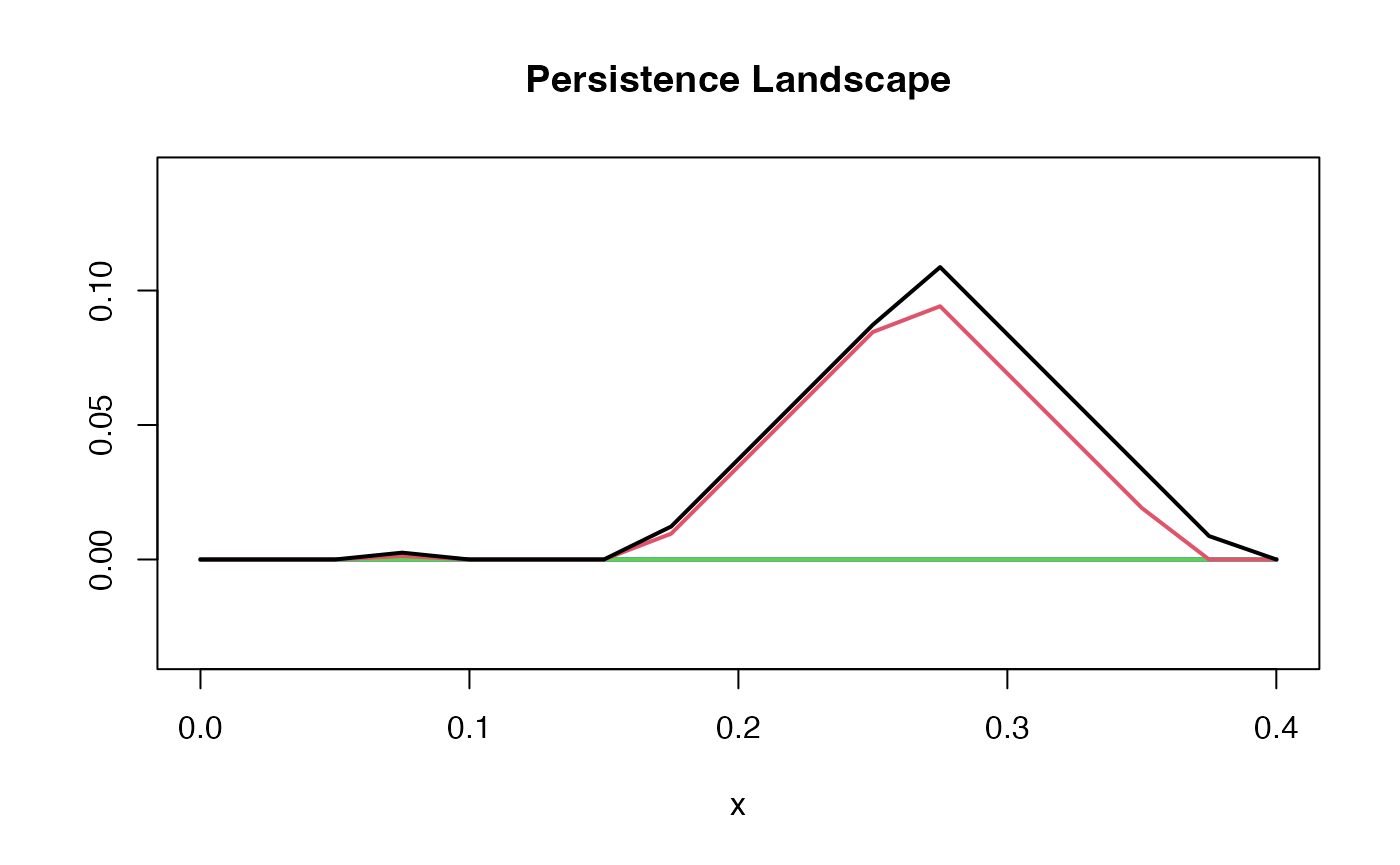

Properties

A persistence landscape has the following properties which make it directly usable for statistical analysis and machine learning:

Stability: Small perturbations in the input data lead to small changes in the landscape, ensuring that results are robust to noise.
Linearity: Persistence landscapes live in a vector space, allowing them to be meaningfully added, scaled, and averaged.
Inner Product Structure: This vector space is in fact a Hilbert space, enabling the definition of distances, norms, and inner products.
Asymptotic Normality: Persistence landscapes satisfy a central limit theorem, enabling the use of normal-distribution-based inference for hypothesis testing and confidence intervals.
Vectorization: Landscapes can be vectorized, making them easily manipulable and compatible with statistical and machine learning pipelines.

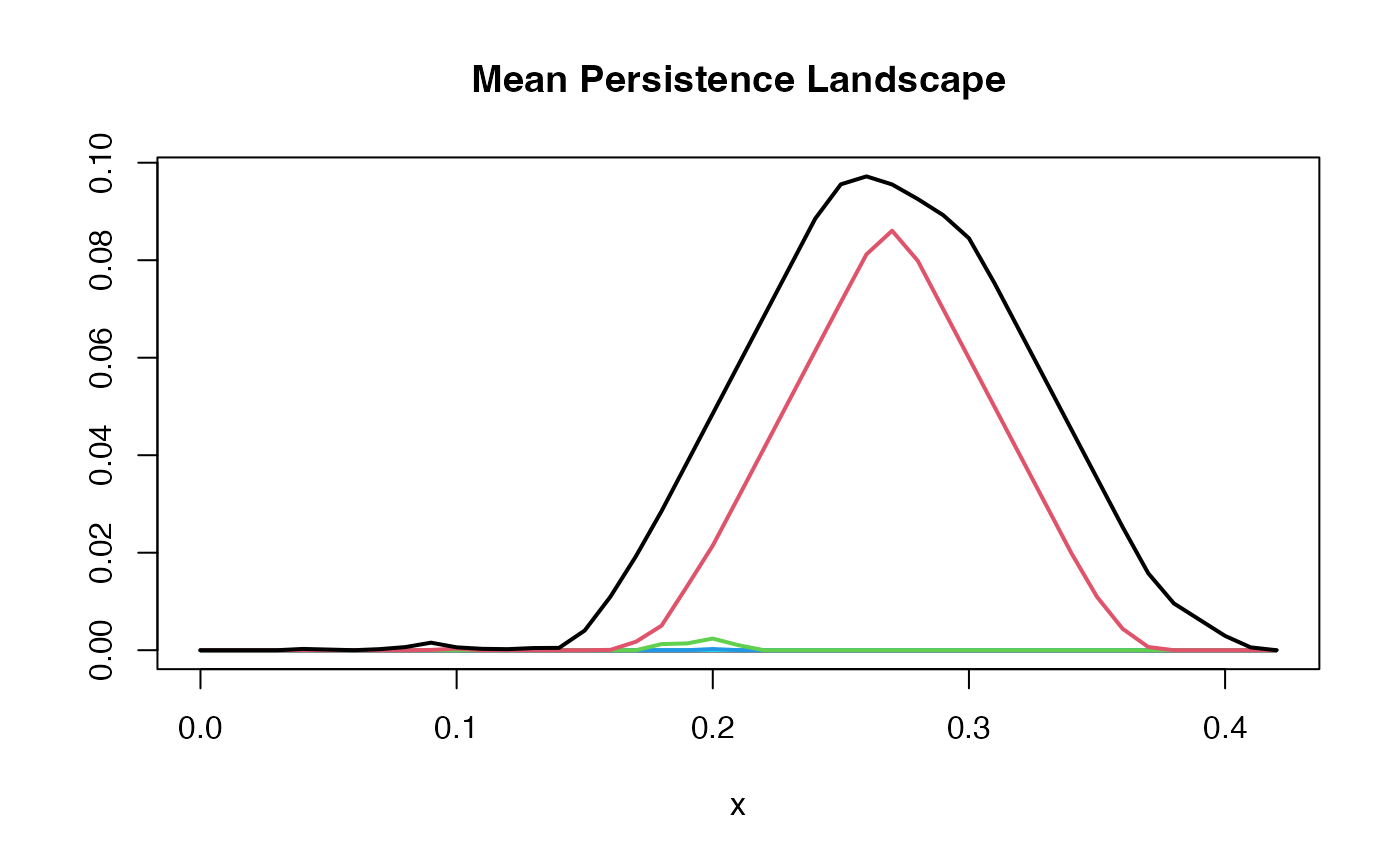
Mean Persistence Landscape

A convenient way of thinking about the mean persistence landscape is by considering its levels. To define a mean on landscapes, we take the pointwise mean of each level. Hence, the mean $i^{\mathbb{th}}$ level is given by $\bar \lambda_i(x) = \frac{1}{N}\sum_{j=1}^{N}\lambda_i ^j(x),$ where $j$ is the index of the landscape, and $N$ is the number of landscapes. Overlaying these mean levels grants us the mean persistence landscape.

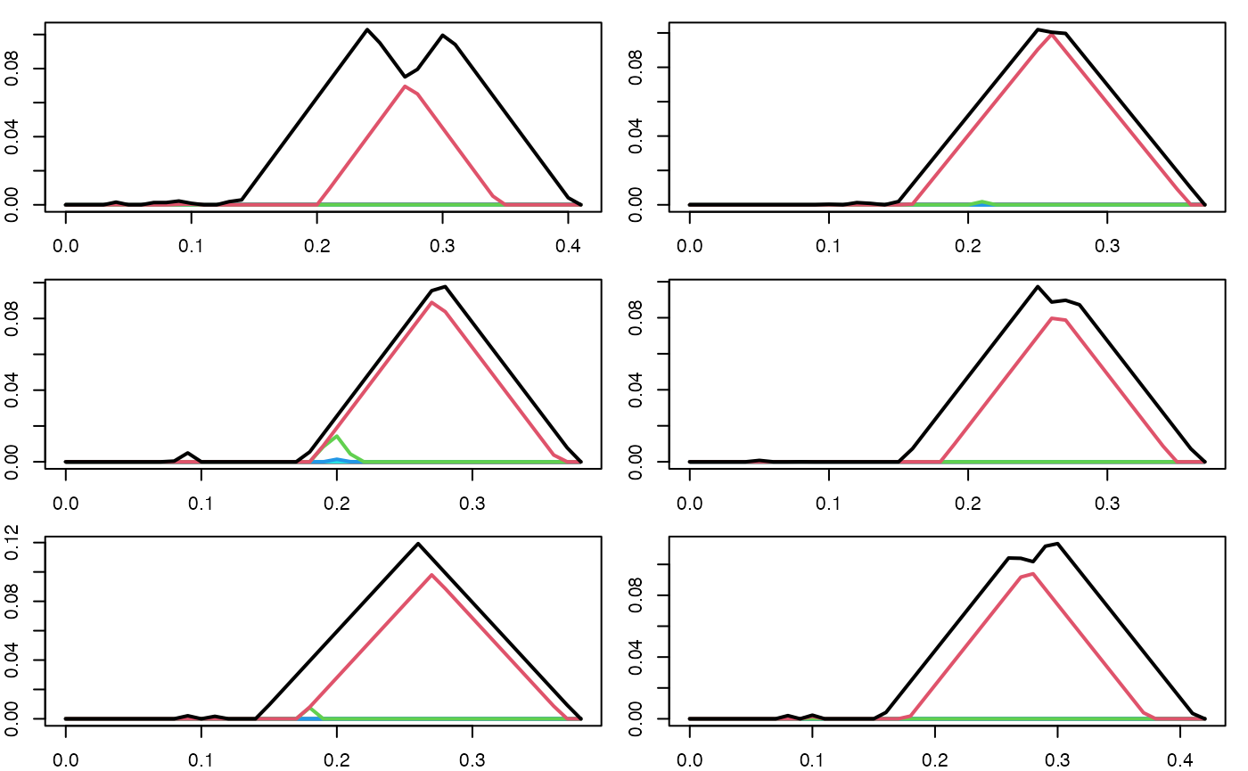
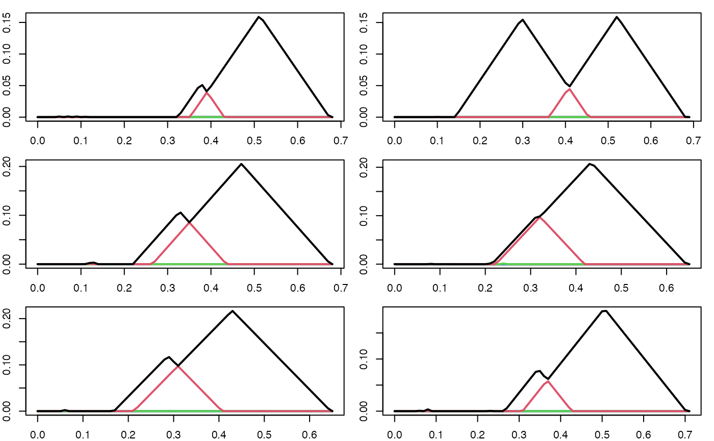
Below, we noisily sample $6$ times from a lemniscate, and then compute the persistence landscape for each sampled point cloud.

set.seed(101137L)
par(mfrow = c(3, 2), mar = c(2,2,1,1))
pl_list_1 <- c()
for (i in seq(6)) {
  pc <- sample_lemniscate_gerono(n = 60, sd = 0.05)
  pd <- alphaComplexDiag(pc, maxdimension = 1)$diagram
  pd[,c(2,3)] <- sqrt(pd[,c(2,3)])
  pl <- pl_new(pd, degree = 1, xby = .01)
  plot(pl)
  pl_list_1 <- c(pl_list_1, pl)
}

We then compute the mean persistence landscape of these $6$ persistence landscapes.

plot(pl_mean(pl_list_1), main = "Mean Persistence Landscape")

Applications of TDA

Hypothesis Testing

In statistics, hypothesis tests are used to weigh the evidence (collected data) to determine whether there is a real effect or phenomenon present in the data, or if its simply a consequence of random sampling or variation. When conducting a hypothesis test, we define a null hypothesis $H_0$ that predicates that no effect is present, and we define an alternative hypothesis $H_A$ that specifies the direction of a present effect. A hypothesis test requires a calculated test statistic from the observed data, and an understanding of the test statistic’s theoretical probability distribution. A $p$ -value is the probability of obtaining a test statistic as extreme or more extreme than the observed test statistic, assuming the null hypothesis to be true. And $\alpha$ , the significance level, is the probability of rejecting the null hypothesis when it is actually true (type I error). This value is typically set by the investigator ahead of time, conventionally to $0.05$ . If the $p < \alpha$ , then we reject our null hypothesis, otherwise we accept or fail to reject it.

In TDA, we can use persistence landscapes to derive test statistics in order to conduct hypotheses tests on samples of point cloud data. Our {plt} hypothesis testing functions — pl_z_test() and pl_perm_test() — provide the test result as a list containing useful information like the estimated distance between the mean landscapes, the test statistic, the $p$ -value, and more. The list is assigned the htest class, which comes with an elegant print() method.

For our next example, we will show how to test whether two collections of point clouds were sampled from different distributions. First, we create a counterfeit lemniscate sampler, which might be similar enough to that of Gerono to, say, deceive a quality control step. This counterfeit lemniscate is the union of differently-sized circles, while the original has same-sized lobes, and it is sampled with noise from the same distribution.

sample_nonsym_lemniscate <- function() {
  circle1 <- circleUnif(n = 25, r = .50)
  circle2 <- circleUnif(n = 35, r = .75)
  
  circle1 <- cbind(circle1[, 1] + 1, circle1[, 2] + 1)
  circle2 <- cbind(circle2[, 1] + 2.25, circle2[, 2] + 1)
  
  circle1 <- add_noise(circle1, sd = 0.05)
  circle2 <- add_noise(circle2, sd = 0.05)
  Y <- rbind(circle1, circle2)
}
plot(sample_nonsym_lemniscate(), asp = 1, pch = 16, xlab = "x", ylab = "y", main = "Non-symmetric Figure Eight Point Cloud")

We noisily sample $6$ times from the lemniscate sampler above, compute the persistence landscape for each point cloud, and then plot the persistence landscapes.

set.seed(194114L)
par(mfrow = c(3, 2), mar = c(2,2,1,1))
pl_list_2 <- c()
for (i in seq(6)) {
  pc <- sample_nonsym_lemniscate()
  pd <- alphaComplexDiag(pc, maxdimension = 1)$diagram
  pd[,c(2,3)] <- sqrt(pd[,c(2,3)])
  pl <- pl_new(pd, degree = 1, xby = .01)
  plot(pl)
  pl_list_2 <- c(pl_list_2, pl)
}

We will refer to the sampling distributions, pl_list_1 and pl_list_2, as $P_1$ and $P_2$ . Below, we replot the mean persistence landscape of $P_1$ (figure eight) and plot the mean persistence landscape of $P_2$ (non-symmetric figure eight). We denote these mean landscapes as $\bar{P_1}$ and $\bar{P_2}$ .

par(mfrow = c(2,1), mar = c(2,2,0.25,2))
plot(pl_mean(pl_list_1))
title("Mean PL of P1", adj = 0.1, line = -1)
plot(pl_mean(pl_list_2))
title("Mean PL of P2", adj = 0.1, line = -1)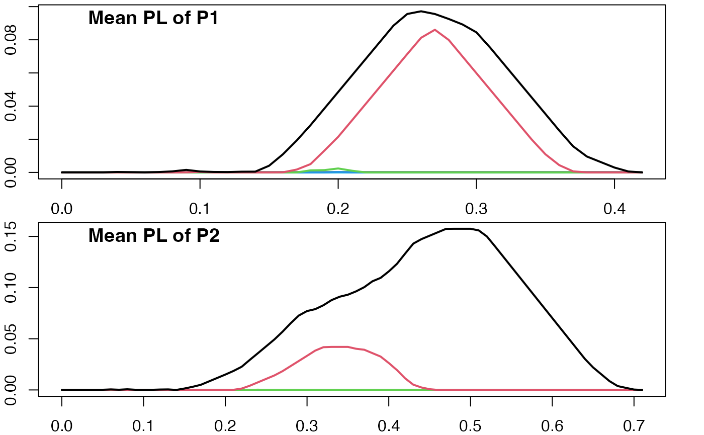

There is a visual difference between the landscapes, but we haven’t quantified the strength of evidence for this difference.

We will use a two sample Z-test and a permutation test to determine if there is a statistically significant difference between $\bar{P_1}$ and $\bar{P_2}$ .

Z-Test

The purpose of a two sample Z-test is to test for the difference of means between two samples from two population distributions. The Z-test is a parametric test that requires the two samples to be normally distributed and performs well when you have large sample sizes and known population variances. If these assumptions are not met, then the test is inappropriate.

To conduct this test on persistent landscapes, the test statistic requires a functional, the integral of the mean persistent landscape, to quantify the difference in mean persistence landscapes. The interval of this integration is determined by the support provided from the user. Specifically, users can enter intervals for the support parameter to focus on regions where important topological features lie, which would increase computational efficiency. The test statistic is $z = \frac{\bar{P_1}-\bar{P_2}}{\sqrt{\frac{S^2_{P_1}}{n_1}+\frac{S^2_{P_2}}{n_2}}},$

where the denominator is the standard error for the difference and $z \sim N(0,1)$ . For more information, please reference section 3 of Bubenik (2015).

In our example, the null hypothesis is that there is not a difference in the two mean persistence landscapes, which would imply that they both came from the same population distribution. And the alternative hypothesis is that there is a difference between the mean persistence landscapes. Succinctly, we test $H_0: \bar{P_1}-\bar{P_2} = 0$ $\text{vs}$ $H_A: \bar{P_1}-\bar{P_2} \ne 0$ .

We can adjust $\alpha$ by changing the conf.level. Here, we will use the default $0.95$ confidence level, so $\alpha=0.05$ . Also, the user can adjust the direction of the alternative hypothesis by setting the alternative argument to “two.sided” (default), “greater” or “less”.

(ztest <- pl_z_test(pl_list_1, pl_list_2, alternative = "two.sided", conf.level = 0.95))
#> 
#>  z-test
#> 
#> data:  
#> z = -2.3495, df = 10, p-value = 0.0188
#> alternative hypothesis: true difference in means is not equal to 0
#> 95 percent confidence interval:
#>  -0.049991074 -0.004518401
#> sample estimates:
#> mean integral of x mean integral of y 
#>         0.02177963         0.04903436

Since the $p$ -value is $0.019$ , we reject the null hypothesis. This result suggests that, according to the Z-test, the samples appear to come from the different distributions, though the evidence was not as strong as we might want. This highlights the Z-test’s conservative nature when testing for differences between two samples of persistence landscapes, especially when we have small sample sizes.

Permutation Test

We now perform a permutation test, which is a non-parametric hypothesis test. This test is useful for smaller sample sizes and does not require an assumption of distribution of the data. Specifically, the principle assumption of the permutation test is that the observations (in our case, the persistence landscapes) do not come from two distinct population distributions $F_{P_1}$ & $F_{P_2}$ , and that they are completely exchangeable across the two groups.

The first step of the permutation test is to calculate an initial test statistic. For our data, it will be $K = \bar{P_1}-\bar{P_2}$ . We build the sampling distribution by rearranging our $12$ samples ( $6$ each from $P_1$ and $P_2$ ) and computing the test statistic for each permutation. We then compare the initial test statistic to the distribution of test statistics we obtained by randomly permuting the data. This helps to determine whether the observed effect is statistically significant.

The null hypothesis is that $P_1$ and $P_2$ come from the same distribution and the alternative hypothesis being that they do not come from the same population distribution. Succinctly, we test $H_0: F_{P_1} = F_{P_2}$ $\text{vs}$ $H_A: F_{P_1} \ne F_{P_2}$ .

(perm <- pl_perm_test(pl_list_1, pl_list_2, complete = TRUE))
#> 
#>  permutation test
#> 
#> data:  
#> p-value = 0.002165
#> alternative hypothesis: true distance between mean landscapes is greater than 0
#> sample estimates:
#> distance between mean landscapes 
#>                       0.06887439

Since the $p$ -value is $0.0022$ , we again reject the null hypothesis. This $p$ -value was an order of magnitude smaller than that obtained from the two sample Z-test. These two hypothesis tests are looking at the data in different ways, so one test may detect the topological (or geometric) difference between the samples more effectively than the other.

Exploratory Dimension Reduction

In this section, we conduct exploratory analysis using variance decomposition. This is done to reduce the dimensions of our data while retaining as much variance as possible. We will use principal components analysis (PCA), which transforms the given variables into a new set of uncorrelated variables called principal components. These components are ordered by the amount of variance they capture from the data, with the first component capturing the most variance, and each subsequent component capturing progressively less. We apply PCA to the vectorized forms of the persistence landscapes.

We continue using the lists from our example. We utilize the pl_to_matrix() function, which converts our persistence landscapes into matrix format, allowing us to perform general-purpose data analytic operations on them. prcomp() performs PCA on our vectorized persistence landscapes.

pl_list <- c(pl_list_1,pl_list_2)
pl_vectors <- pl_to_matrix(pl_list)
pca <- prcomp(pl_vectors)
plot(pca, type = "l", main = "Scree Plot")

summary(pca)
#> Importance of components:
#>                           PC1    PC2     PC3     PC4     PC5     PC6     PC7
#> Standard deviation     0.3681 0.1559 0.10456 0.03776 0.03496 0.02385 0.02245
#> Proportion of Variance 0.7749 0.1390 0.06254 0.00815 0.00699 0.00325 0.00288
#> Cumulative Proportion  0.7749 0.9140 0.97649 0.98465 0.99164 0.99489 0.99777
#>                            PC8     PC9     PC10     PC11      PC12
#> Standard deviation     0.01361 0.01097 0.007923 0.004584 4.883e-17
#> Proportion of Variance 0.00106 0.00069 0.000360 0.000120 0.000e+00
#> Cumulative Proportion  0.99883 0.99952 0.999880 1.000000 1.000e+00

In the summary above, we see that about $77.5\%$ of the variance in the original data is captured in the first principal component, and about $13.9\%$ of the variance is captured in the second principal component. So the first and second principal component are sufficient to explain the variance of the data.

To evaluate whether the dimension reduction was successful, we assign labels to our data based on the distribution they were generated from and plot each sample with their corresponding first principal component and second principal component values to see if any clustering or patterns occurred.

data.labels <- c(rep(1,length(pl_list_1)), rep(2,length(pl_list_2)))
plot(pca$x[,1:2], col = data.labels, pch = 17 + (2 * data.labels), asp = 1)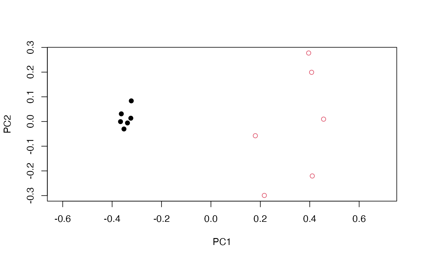

As we can see, clustering of samples from the same sample did occur. We observe that the between-group variance is mainly contained in the first principal component. Also, the within-group variance of $P_1$ is smaller than the between-group variance of $P_2$ .

Classification

We now build a machine learning model to classify the point clouds using their vectorized persistence landscapes. A support vector machine (SVM) is a supervised algorithm commonly used for classification tasks. It works by finding the optimal hyperplane that best separates the classes ( $P_1$ or $P_2$ ) in the feature space (where each dimension of the feature space corresponds to one of the elements in these vectors), maximizing the margin between the closest data points of each class, known as support vectors.

Below we train our model using svm() and perform $4$ -fold cross validation. That is, the algorithm splits the data into $4$ groups and as it iterates to using each group as the testing group, it uses the other $3$ groups as the training data. We set scale = FALSE so that more persistent features have more weight.

svm_model <- svm(pl_vectors,data.labels,scale = FALSE,
                 type = "C-classification", kernel = "linear", cost = 10, cross = 4)
summary(svm_model)
#> 
#> Call:
#> svm.default(x = pl_vectors, y = data.labels, scale = FALSE, type = "C-classification", 
#>     kernel = "linear", cost = 10, cross = 4)
#> 
#> 
#> Parameters:
#>    SVM-Type:  C-classification 
#>  SVM-Kernel:  linear 
#>        cost:  10 
#> 
#> Number of Support Vectors:  3
#> 
#>  ( 1 2 )
#> 
#> 
#> Number of Classes:  2 
#> 
#> Levels: 
#>  1 2
#> 
#> 4-fold cross-validation on training data:
#> 
#> Total Accuracy: 100 
#> Single Accuracies:
#>  100 100 100 100

The model successfully distinguishes between the different topological structures present in the two persistence landscapes.

Supporting Information

Appendix

A $k$ -simplex is a $k$ -dimensional polytope which is the convex hull of $k+1$ points in Euclidean space in general position (the points $x_1,...,x_{k+1}$ are affinely independent, which means that the vectors $x_2-x_1,...,x_{k+1}-x_1$ are linearly independent). The convex hull of a non-empty subset of these points is called the face of the simplex.

A simplicial complex is a set $K$ of simplices such that

the face of any simplex in $K$ is also in $K$ ; and
any non-empty intersection of two simplices is a face of both of them.

An abstract simplicial complex is a set $K$ of non-empty subsets of a fixed set such that if $A \in K$ , then all nonempty subsets of $A$ are also in $K$ .

For a finite set of points $X \subset \mathbb{R}^d$ , the Alpha complex Alpha $(X,s)$ is a simplicial subcomplex of the Delaunay complex of $X$ consisting of simplices of circumradius less than or equal to $\sqrt{s}$ . The Alpha complex is defined as: $\text{Alpha}(X, r) = \{ \sigma \subset X : \bigcap_{u \in \sigma} R_u(\sqrt{s}) \neq \emptyset \}.$

A filtered simplicial complex consists of a nested sequence of simplicial complexes: $K_0 \subset K_1 \subset K_2 \subset \;...\subset K_n$

Applying homology, we obtain a sequence of vector spaces and linear maps called a persistence module: $H_k(K_0) \rightarrow H_k(K_1) \rightarrow H_k(K_2) \rightarrow \;...\rightarrow H_k(K_n)$ The images of these maps and compositions of these maps are called persistence homology vector spaces.

A persistence module $M$ consists of a vector space $M_a$ for all $a \in \mathbb{R}$ and linear maps $M(a\leq b):M_a \to M_b$ for all $a \leq b$ such that $M(a \leq a)$ is the identity map and for all $a \leq b \leq c, \; M(b \leq c) \circ M(a \leq b) = M (a \leq c)$ .

Let $M$ be a persistence module and $b_i \leq d_i$ where $b_i$ is some birth value and $d_i$ is some death value. The betti number of $M$ is $\beta^{b_i, d_i} = \dim(\text{im}(M(b_i \leq d_i)))$

The $k^{th}$ Betti number, $\beta_k$ , counts the number of $k$ -dimensional features of a simplicial complex. For example, $\beta_0$ counts the number of connected components and $\beta_1$ counts the number of holes.

The rank function, $\lambda: \mathbb{R}^2 \rightarrow \mathbb{R}$ defined as: $\mathbb{\lambda}(b, d) = \begin{cases} \mathbb{\beta}^{(b,d)} & \text{if } d \geq b \\ 0 & \text{otherwise} \end{cases}$

Now, we change the coordinate system from (birth, death) scale to the (midlife, halflife) scale for ease of interpretability and analysis. We have: $m = \frac{(b + d)}{ 2} \; \text{and} \;h = \frac{(d-b)}{2}.$ Hence our rescaled rank function, $\mathbb{\lambda}: \mathbb{R}^2 \rightarrow \mathbb{R}$ , defined as:
$\mathbb{\lambda}(m, h) = \begin{cases} \mathbb{\beta}^{(m-h,m+h)} & \text{if } h \geq 0 \\ 0 & \text{otherwise} \end{cases}$ .

Finally, the persistence landscape is a function, $\lambda: \mathbb{N} \times \mathbb{R} \rightarrow \mathbb{R}$ . Or it could be thought of as a sequence of functions $\lambda_k: \mathbb{R} \to \mathbb{R}$ , where $\lambda_k(t) = \lambda(k,t)$ . $\lambda_k(t)$ is defined as: $\lambda_k(t) = \sup(m \geq 0 | \beta^{t-m, t+m} \geq k)$ Essentially, $\lambda_k(t)$ finds the largest interval around t where there at least $k$ persistent features.

References

Bubenik, Peter. “Statistical Topological Data Analysis Using Persistence Landscapes.” Journal of Machine Learning Research, vol. 16, 2015, pp. 77-102.↩︎
https://people.clas.ufl.edu/peterbubenik/intro-to-tda/↩︎

James Golabek, Aidan Bryant, Jason Cory Brunson, Johnathan Bush, Iryna Hartsock, Peter Bubenik