Represent log-ratios between variables based on their values on a population of cases.
Usage
lra(x, compositional = FALSE, weighted = TRUE)

# S3 method for class 'lra'
print(x, nd = length(x$sv), n = 6L, ...)

# S3 method for class 'lra'
screeplot(x, main = deparse1(substitute(x)), ...)

# S3 method for class 'lra'
biplot(
  x,
  choices = c(1L, 2L),
  scale = c(0, 0),
  main = deparse1(substitute(x)),
  var.axes = FALSE,
  ...
)

# S3 method for class 'lra'
plot(x, main = deparse1(substitute(x)), ...)
Arguments
- x
A numeric matrix or rectangular data set.
- compositional
Logical; whether to normalize rows of
xto sum to 1.- weighted
Logical; whether to weight rows and columns by their sums.
- nd
Integer; number of shared dimensions to include in print.
- n
Integer; number of rows of each factor to print.
- main, var.axes, ...
Parameters passed to other plotting methods (in the case of
main, after beingforce()d.- choices
Integer; length-2 vector specifying the components to plot.
- scale
Numeric; values between 0 and 1 that control how inertia is conferred unto the points: Row (
i = 1L) and column (i = 2L) coordinates are scaled bysv ^ scale[[i]]. If a single valuescaleis passed, it is assigned to the rows while1 - scaleis assigned to the columns.
Value
Given an \(n * p\) data matrix and setting \(r=min(n,p)\),
lra() returns a list of class "lra" containing three elements:
svThe \(r-1\) singular values
row.coordsThe \(n * (r-1)\) matrix of row standard coordinates.
column.coordsThe \(p * (r-1)\) matrix of column standard coordinates.
row.weightsThe weights used to scale the row coordinates.
column.weightsThe weights used to scale the column coordinates.
Details
Log-ratio analysis (LRA) is based on a double-centering of log-transformed data, usually weighted by row and column totals. The technique is suitable for positive-valued variables on a common scale (e.g. percentages). The distances between variables' coordinates (in the full-dimensional space) are their pairwise log-ratios. The distances between cases' coordinates are called their log-ratio distances, and the total variance is the weighted sum of their squares.
LRA is not implemented in standard R distributions but is a useful member of the ordination toolkit. This is a minimal implementation following Greenacre's (2010) exposition in Chapter 7.
References
Greenacre MJ (2010) Biplots in Practice. Fundacion BBVA, ISBN: 978-84-923846. https://www.fbbva.es/microsite/multivariate-statistics/biplots.html
Examples
# U.S. 1973 violent crime arrests
head(USArrests)
#>            Murder Assault UrbanPop Rape
#> Alabama      13.2     236       58 21.2
#> Alaska       10.0     263       48 44.5
#> Arizona       8.1     294       80 31.0
#> Arkansas      8.8     190       50 19.5
#> California    9.0     276       91 40.6
#> Colorado      7.9     204       78 38.7
# row and column subsets
state_examples <- c("Hawaii", "Mississippi", "North Dakota")
arrests <- c(1L, 2L, 4L)

# pairwise log-ratios of violent crime arrests for two states
arrest_pairs <- combn(arrests, 2L)
arrest_ratios <-
  USArrests[, arrest_pairs[1L, ]] / USArrests[, arrest_pairs[2L, ]]
colnames(arrest_ratios) <- paste(
  colnames(USArrests)[arrest_pairs[1L, ]], "/",
  colnames(USArrests)[arrest_pairs[2L, ]], sep = ""
)
arrest_logratios <- log(arrest_ratios)
arrest_logratios[state_examples, ]
#>              Murder/Assault Murder/Rape Assault/Rape
#> Hawaii            -2.160935 -1.33797578    0.8229588
#> Mississippi       -2.778009 -0.06025919    2.7177496
#> North Dakota      -4.029806 -2.21101790    1.8187881

# non-compositional log-ratio analysis
(arrests_lra <- lra(USArrests[, arrests]))
#> Singular values: 0.11758785 0.06383505
#>
#> Row scores (6 of 50):
#>                 LRSV1      LRSV2
#> Alabama    -0.6800120  0.9296011
#> Alaska      0.9299899 -0.6245772
#> Arizona    -0.3298496 -1.3115817
#> Arkansas   -0.3513443  0.2773231
#> California  0.5516590 -1.0042801
#> Colorado    1.2291066 -0.6388469
#>
#> Column scores:
#>             LRSV1      LRSV2
#> Murder   0.283086  4.9570302
#> Assault -0.370595 -0.1805698
#> Rape     2.876702 -0.3660163
screeplot(arrests_lra)

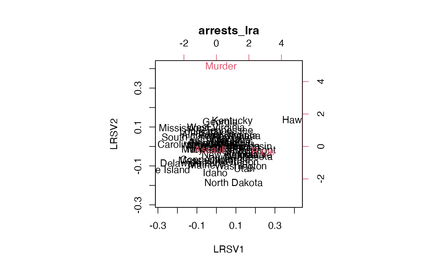
biplot(arrests_lra, scale = c(1, 0), cex = c(2/3, 1))


# compositional log-ratio analysis
(arrests_lra <- lra(USArrests[, arrests], compositional = TRUE))
#> Singular values: 0.12786989 0.07009419
#>
#> Row scores (6 of 50):
#>                 LRSV1      LRSV2
#> Alabama    -0.8599661  1.0266703
#> Alaska      0.6256391 -0.5908842
#> Arizona    -0.5965504 -1.0524702
#> Arkansas   -0.5672002  0.3924046
#> California  0.2531761 -0.8868744
#> Colorado    0.9102533 -0.6422862
#>
#> Column scores:
#>              LRSV1      LRSV2
#> Murder   0.6072392  4.9382810
#> Assault -0.3999883 -0.1533148
#> Rape     2.7051937 -0.5351457
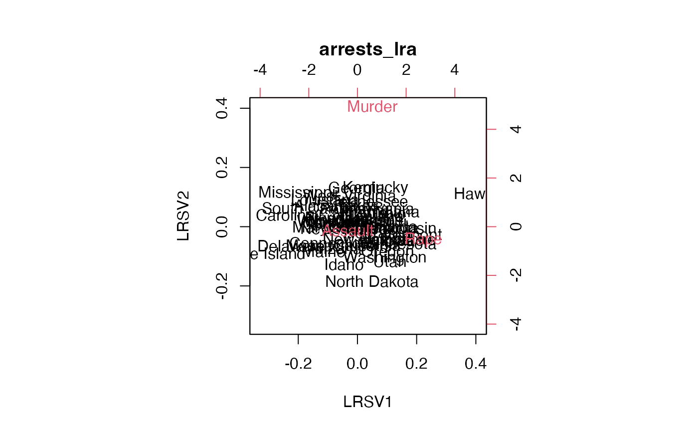
biplot(arrests_lra, scale = c(1, 0), cex = c(2/3, 1))
