The Order of the Rectangles
Jason Cory Brunson
2025-06-12
Source:vignettes/order-rectangles.rmd
order-rectangles.rmdHow the strata and lodes at each axis are ordered, and how to control their order, is a complicated but essential part of {ggalluvial}’s functionality. This vignette explains the motivations behind the implementation and explores the functionality in greater detail than the examples.
Setup
knitr::opts_chunk$set(fig.width = 6, fig.height = 3, fig.align = "center")
library(ggalluvial)
## Loading required package: ggplot2All of the functionality discussed in this vignette is exported by
{ggalluvial}. We’ll also need a toy data set to play with. I conjured
the data frame toy to be nearly as small as possible while
complex enough to illustrate the positional controls:
# toy data set
set.seed(0)
toy <- data.frame(
  subject = rep(LETTERS[1:5], times = 4),
  collection = rep(1:4, each  = 5),
  category = rep(
    sample(c("X", "Y"), 16, replace = TRUE),
    rep(c(1, 2, 1, 1), times = 4)
  ),
  class = c("one", "one", "one", "two", "two")
)
print(toy)
## subject collection category class
## 1 A 1 Y one
## 2 B 1 X one
## 3 C 1 X one
## 4 D 1 Y two
## 5 E 1 X two
## 6 A 2 X one
## 7 B 2 Y one
## 8 C 2 Y one
## 9 D 2 X two
## 10 E 2 X two
## 11 A 3 X one
## 12 B 3 Y one
## 13 C 3 Y one
## 14 D 3 Y two
## 15 E 3 X two
## 16 A 4 X one
## 17 B 4 X one
## 18 C 4 X one
## 19 D 4 X two
## 20 E 4 X twoThe subjects are classified into categories at each collection point but are also members of fixed classes. Here’s how {ggalluvial} visualizes these data under default settings:
ggplot(toy, aes(x = collection, stratum = category, alluvium = subject)) +
  geom_alluvium(aes(fill = class)) +
  geom_stratum()
Motivations
The amount of control the stat layers stat_alluvial()
and stat_flow() exert over the positional
aesthetics of graphical objects (grobs) is unusual, by the standards
of {ggplot2} and many of its extensions. In the
layered grammar of graphics framework, the role of a statistical
transformation is usually to summarize the original data, for example by
binning (stat_bin()) or by calculating quantiles
(stat_qq()). These transformed data are then sent to geom
layers for positioning. The positions of grobs may be adjusted after the
statistical transformation, for example when points are jittered
(geom_jitter()), but the numerical data communicated by the
plot are still the product of the stat.
In {ggalluvial}, the stat layers exert slightly more control. For one
thing, the transformation is more sophisticated than a single value or a
fixed-length vector, such as a mean, standard deviation, or five-number
summary. Instead, the values of y (which default to
1) within each collection are, after reordering,
transformed using cumsum() and some additional arithmetic
to obtain coordinates for the centers y and lower and upper
limits ymin and ymax of the strata
representing the categories. Additionally, the reordering of lodes
within each collection relies on a hierarchy of sorting variables, based
on the strata at nearby axes as well as the present one and, optionally,
on the values of differentiation aesthetics like fill. How
this hierarchy is invoked depends on the choices of several plotting
parameters (decreasing, reverse, and
absolute). Thus, the results of the statistical
transformations are not as intrinsically meaningful as others and are
subject to much more intervention by the user. Only once the
transformations have produced these coordinates do the geom layers use
them to position the rectangles and splines that constitute the
plot.
There are two key reasons for this division of labor:
- The coordinates returned by some stat layers can be coupled with
multiple geom layers. For example, all four geoms can couple with the
alluviumstat. Moreover, as showcased in the examples, the stats can also meaningfully couple with exogenous geoms liketext,pointrange, anderrorbar. (In principle, the geoms could also couple with exogenous stats, but i haven’t done this or seen it done in the wild.) - Different parameters control the calculations of the coordinates
(e.g.
aes.bindandcement.alluvia) and the rendering of the graphical elements (width,knot.pos, andaes.flow), and it makes intuitive sense to handle these separately. For example, the heights of the strata and lodes convey information about the underlying data, whereas their widths are arbitrary.
(If the data are provided in alluvia format, then
Stat*$setup_data() converts them to lodes format in
preparation for the main transformation. This can be done manually using
the
exported conversion functions, and this vignette will assume the
data are already in lodes format.)
Positioning strata
Each stat layer demarcates one stack for each data collection point and one rectangle within each stack for each (non-empty) category.1 In {ggalluvial} terms, the collection points are axes and the rectangles are strata or lodes.
To generate a sequence of stacked bar plots with no connecting flows,
only the aesthetics x (standard) and stratum
(custom) are required:
# collection point and category variables only
data <- structure(toy[, 2:3], names = c("x", "stratum"))
# required fields for stat transformations
data$y <- 1
data$PANEL <- 1
# stratum transformation
StatStratum$compute_panel(data)
## x stratum y n count deposit prop ymin ymax
## 2 1 Y 1.0 2 2 1 0.4 0 2
## 1 1 X 3.5 3 3 2 0.6 2 5
## 4 2 Y 1.0 2 2 3 0.4 0 2
## 3 2 X 3.5 3 3 4 0.6 2 5
## 6 3 Y 1.5 3 3 5 0.6 0 3
## 5 3 X 4.0 2 2 6 0.4 3 5
## 7 4 X 2.5 5 5 7 1.0 0 5Comparing this output to toy, notice first that the data
have been aggregated: Each distinct combination of x and
stratum occupies only one row. x encodes the
axes and is subject to layers specific to this positional aesthetic,
e.g. scale_x_*() transformations. ymin and
ymax are the lower and upper bounds of the rectangles, and
y is their vertical centers. Each stacked rectangle begins
where the one below it ends, and their heights are the numbers of
subjects (or the totals of their y values, if
y is passed a numerical variable) that take the
corresponding category value at the corresponding collection point.
Here’s the plot this strata-only transformation yields:
ggplot(toy, aes(x = collection, stratum = category)) +
  stat_stratum() +
  stat_stratum(geom = "text", aes(label = category))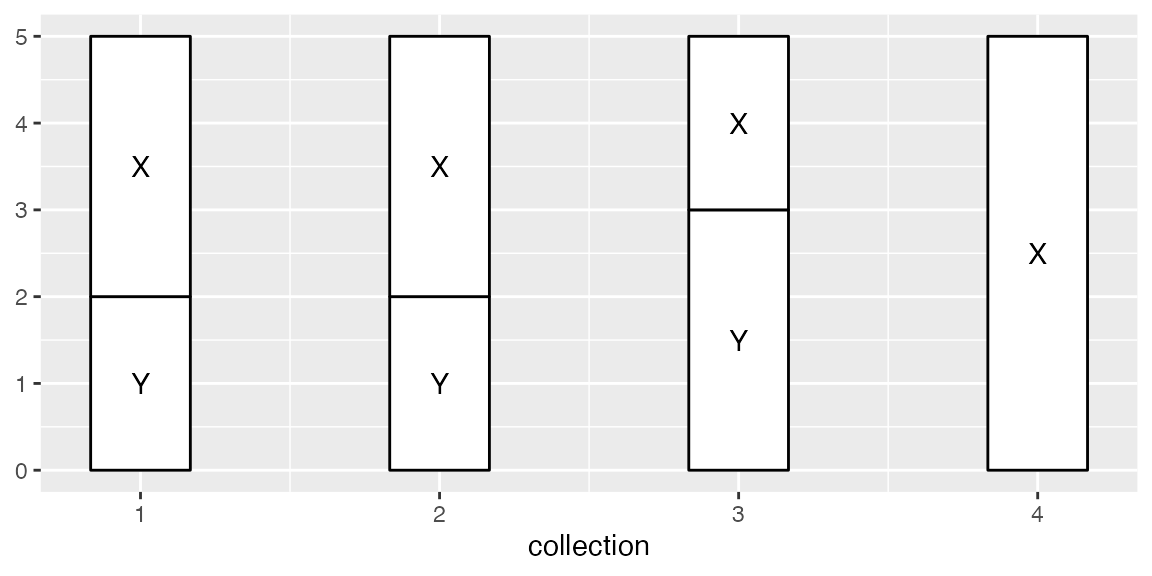
In this vignette, i’ll use the stat_*() functions to add
layers, so that the parameters that control their behavior are
accessible via tab-completion.
Reversing the strata
Within each axis, stratum defaults to reverse order so
that the bars proceed in the original order from top to bottom. This can
be overridden by setting reverse = FALSE in
stat_stratum():
# stratum transformation with strata in original order
StatStratum$compute_panel(data, reverse = FALSE)
## x stratum y n count deposit prop ymin ymax
## 1 1 X 1.5 3 3 1 0.6 0 3
## 2 1 Y 4.0 2 2 2 0.4 3 5
## 3 2 X 1.5 3 3 3 0.6 0 3
## 4 2 Y 4.0 2 2 4 0.4 3 5
## 5 3 X 1.0 2 2 5 0.4 0 2
## 6 3 Y 3.5 3 3 6 0.6 2 5
## 7 4 X 2.5 5 5 7 1.0 0 5
ggplot(toy, aes(x = collection, stratum = category)) +
  stat_stratum(reverse = FALSE) +
  stat_stratum(geom = "text", aes(label = category), reverse = FALSE)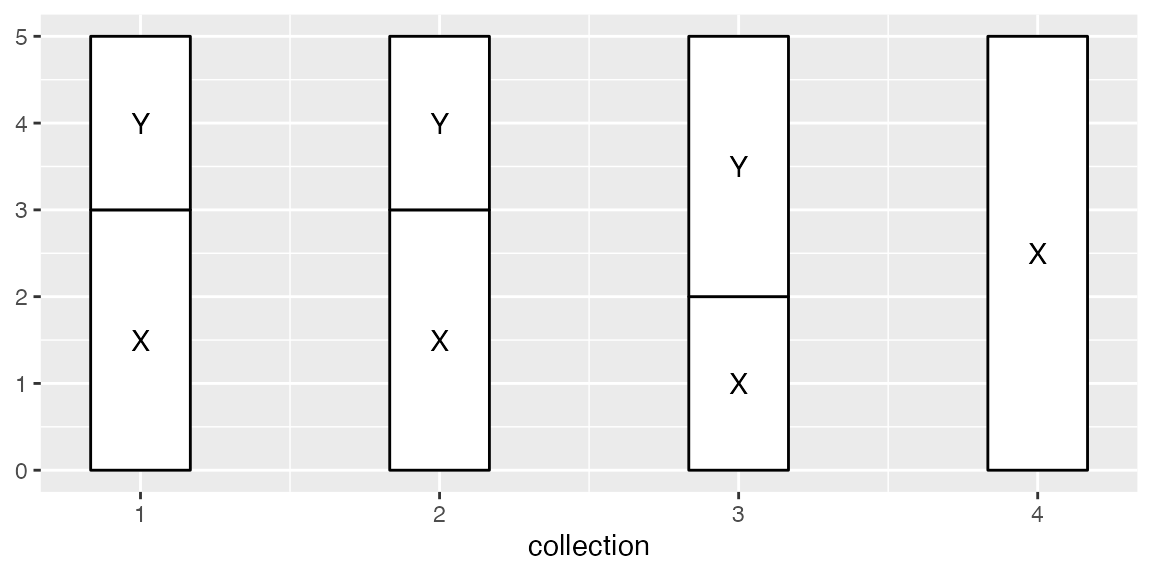
Warning: The caveat to this is that, if
reverse is declared in any layer, then it must be declared
in every layer, lest the layers be misaligned. This includes any
alluvium, flow, and lode layers,
since their graphical elements are organized within the bounds of the
strata.
Sorting the strata by size
When the strata are defined by a character or factor variable, they
default to the order of the variable (lexicographic in the former case).
This can be overridden by the decreasing parameter, which
defaults to NA but can be set to TRUE or
FALSE to arrange the strata in decreasing or increasing
order in the y direction:
# stratum transformation with strata in original order
StatStratum$compute_panel(data, reverse = FALSE)
## x stratum y n count deposit prop ymin ymax
## 1 1 X 1.5 3 3 1 0.6 0 3
## 2 1 Y 4.0 2 2 2 0.4 3 5
## 3 2 X 1.5 3 3 3 0.6 0 3
## 4 2 Y 4.0 2 2 4 0.4 3 5
## 5 3 X 1.0 2 2 5 0.4 0 2
## 6 3 Y 3.5 3 3 6 0.6 2 5
## 7 4 X 2.5 5 5 7 1.0 0 5
ggplot(toy, aes(x = collection, stratum = category)) +
  stat_stratum(decreasing = TRUE) +
  stat_stratum(geom = "text", aes(label = category), decreasing = TRUE)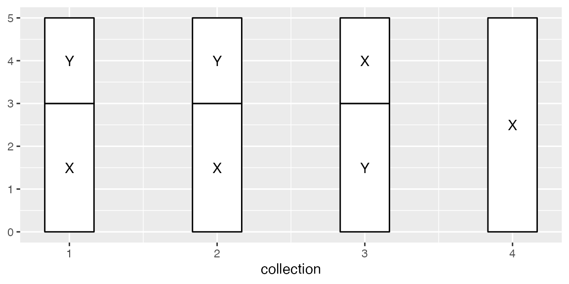
Warning: The same caveat applies to
decreasing as to reverse: Make sure that all
layers using alluvial stats are passed the same values! Henceforth,
we’ll use the default (reverse and categorical) ordering of the strata
themselves.
Positioning lodes within strata
Alluvia and flows
In the strata-only plot, each subject is represented once at each
axis. Alluvia are x-splines that connect these multiple
representations of the same subjects across the axes. In order to avoid
having these splines overlap at the axes, the alluvium stat
must stack the alluvial cohorts—subsets of subjects who have a common
profile across all axes—within each stratum. These smaller
cohort-specific rectangles are the lodes. This calculation
requires the additional custom alluvium aesthetic, which
identifies common subjects across the axes:
# collection point, category, and subject variables
data <- structure(toy[, 1:3], names = c("alluvium", "x", "stratum"))
# required fields for stat transformations
data$y <- 1
data$PANEL <- 1
# alluvium transformation
StatAlluvium$compute_panel(data)
## x alluvium stratum y PANEL lode n count deposit prop ymin ymax group
## 1 1 A Y 1.5 1 A 1 1 1 0.2 1 2 1
## 2 1 B X 3.5 1 B 1 1 2 0.2 3 4 2
## 3 1 C X 2.5 1 C 1 1 2 0.2 2 3 3
## 4 1 D Y 0.5 1 D 1 1 1 0.2 0 1 4
## 5 1 E X 4.5 1 E 1 1 2 0.2 4 5 5
## 6 2 A X 3.5 1 A 1 1 4 0.2 3 4 1
## 7 2 B Y 1.5 1 B 1 1 3 0.2 1 2 2
## 8 2 C Y 0.5 1 C 1 1 3 0.2 0 1 3
## 9 2 D X 2.5 1 D 1 1 4 0.2 2 3 4
## 10 2 E X 4.5 1 E 1 1 4 0.2 4 5 5
## 11 3 A X 3.5 1 A 1 1 6 0.2 3 4 1
## 12 3 B Y 1.5 1 B 1 1 5 0.2 1 2 2
## 13 3 C Y 0.5 1 C 1 1 5 0.2 0 1 3
## 14 3 D Y 2.5 1 D 1 1 5 0.2 2 3 4
## 15 3 E X 4.5 1 E 1 1 6 0.2 4 5 5
## 16 4 A X 3.5 1 A 1 1 7 0.2 3 4 1
## 17 4 B X 1.5 1 B 1 1 7 0.2 1 2 2
## 18 4 C X 0.5 1 C 1 1 7 0.2 0 1 3
## 19 4 D X 2.5 1 D 1 1 7 0.2 2 3 4
## 20 4 E X 4.5 1 E 1 1 7 0.2 4 5 5The transformed data now contain one row per cohort—instead
of per category—per collection point. The vertical positional
aesthetics describe the lodes rather than the strata, and the
group variable encodes the alluvia (a
convenience for the geom layer, and the reason that {ggalluvial} stat
layers ignore variables passed to group).
Here’s how this transformation translates into the alluvial plot that began the vignette, labeling the subject of each alluvium at each intersection with a stratum:
ggplot(toy, aes(x = collection, stratum = category, alluvium = subject)) +
  stat_alluvium(aes(fill = class)) +
  stat_stratum(alpha = .25) +
  stat_alluvium(geom = "text", aes(label = subject))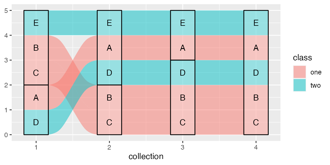
The flow stat differs from the alluvium
stat by allowing the orders of the lodes within strata to differ from
one side of an axis to the other. Put differently, the flow
stat allows mixing at the axes, rather than requiring that each
case or cohort is follows a continuous trajectory from one end of the
plot to the other. As a result, flow plots are often much less
cluttered, the trade-off being that cases or cohorts cannot be tracked
through them.
# flow transformation
StatFlow$compute_panel(data)
## alluvium x stratum deposit flow y n count lode group prop ymin ymax
## 3 2 1 Y 1 from 1.0 2 2 A 2 0.4 0 2
## 1 1 1 X 2 from 3.0 2 2 B 1 0.4 2 4
## 5 3 1 X 2 from 4.5 1 1 E 3 0.2 4 5
## 2 1 2 Y 3 to 1.0 2 2 B 1 0.2 0 2
## 4 2 2 X 4 to 3.0 2 2 A 2 0.2 2 4
## 6 3 2 X 4 to 4.5 1 1 E 3 0.1 4 5
## 7 4 2 Y 3 from 1.0 2 2 B 4 0.2 0 2
## 9 5 2 X 4 from 2.5 1 1 D 5 0.1 2 3
## 11 6 2 X 4 from 4.0 2 2 A 6 0.2 3 5
## 8 4 3 Y 5 to 1.0 2 2 B 4 0.2 0 2
## 10 5 3 Y 5 to 2.5 1 1 D 5 0.1 2 3
## 12 6 3 X 6 to 4.0 2 2 A 6 0.2 3 5
## 13 7 3 Y 5 from 1.5 3 3 B 7 0.3 0 3
## 15 8 3 X 6 from 4.0 2 2 A 8 0.2 3 5
## 14 7 4 X 7 to 1.5 3 3 B 7 0.6 0 3
## 16 8 4 X 7 to 4.0 2 2 A 8 0.4 3 5The flow stat transformation yields one row per
cohort per side per flow. Each intermediate axis appears twice in
the data, once for the incoming flow and once for the outgoing flow.
(The starting and ending axes only have rows for outgoing and incoming
flows, respectively.) Here is the flow version of the preceding alluvial
plot, labeling each side of each flow with the corresponding
subject:
ggplot(toy, aes(x = collection, stratum = category, alluvium = subject)) +
  stat_stratum() +
  stat_flow(aes(fill = class)) +
  stat_flow(geom = "text",
            aes(label = subject, hjust = after_stat(flow) == "to"))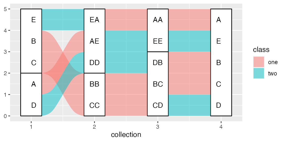
The computed
variable flow indicates whether each row of the
compute_panel() output corresponds to a flow to or
from its axis; the values are used to nudge the labels toward
their respective flows (to avoid overlap). Mismatches between adjacent
labels indicate where lodes are ordered differently on either side of a
stratum.
Lode guidance
As the number of strata at each axis grows, heterogeneous cases or cohorts can produce highly complex alluvia and very messy plots. {ggalluvial} mitigates this by strategically arranging the lodes—the intersections of the alluvia with the strata—so as to reduce their crossings between adjacent axes. This strategy is executed locally: At each axis (call it the index axis), the order of the lodes is guided by several totally or partially ordered variables. In order of priority:
- the strata at the index axis
- the strata at the other axes to which the index axis is linked by alluvia or flows—namely, all other axes in the case of an alluvium, or a single adjacent axis in the case of a flow
- the alluvia themselves, i.e. the variable passed to
alluvium
In the alluvium case, the prioritization of the remaining axes is
determined by a lode guidance function. A lode guidance
function can be passed to the lode.guidance parameter,
which defaults to "zigzag". This function puts the nearest
(adjacent) axes first, then zigzags outward from there, initially (the
“zig”) in the direction of the closer extreme:
for (i in 1:4) print(lode_zigzag(4, i))## [1] 1 2 3 4
## [1] 2 1 3 4
## [1] 3 4 2 1
## [1] 4 3 2 1Several alternative lode_*() functions are
available:
-
"zagzig"behaves like"zigzag"except initially “zags” toward the farther extreme. -
"frontback"and"backfront"behave like"zigzag"but extend completely in one outward direction from the index axis before the other. -
"forward"and"backward"put the remaining axes in increasing and decreasing order, regardless of the relative position of the index axis.
Two alternatives are illustrated below:
for (i in 1:4) print(lode_backfront(4, i))## [1] 1 2 3 4
## [1] 2 1 3 4
## [1] 3 2 1 4
## [1] 4 3 2 1
ggplot(toy, aes(x = collection, stratum = category, alluvium = subject)) +
  stat_alluvium(aes(fill = class), lode.guidance = "backfront") +
  stat_stratum() +
  stat_alluvium(geom = "text", aes(label = subject),
                lode.guidance = "backfront")
The difference between "backfront" guidance and
"zigzag" guidance can be seen in the order of the lodes of
the "Y" stratum at axis 3: Whereas
"zigzag" minimized the crossings between axes
3 and 4, locating the distinctive
class-"one" case above the others, "backfront"
minimized the crossings between axes 2 and 3
(axis 2 being immediately before axis 3),
locating this case below the others.
for (i in 1:4) print(lode_backward(4, i))## [1] 1 4 3 2
## [1] 2 4 3 1
## [1] 3 4 2 1
## [1] 4 3 2 1
ggplot(toy, aes(x = collection, stratum = category, alluvium = subject)) +
  stat_alluvium(aes(fill = class), lode.guidance = "backward") +
  stat_stratum() +
  stat_alluvium(geom = "text", aes(label = subject),
                lode.guidance = "backward")
The effect of "backward" guidance is to keep the right
part of the plot as tidy as possible while allowing the left part to
become as messy as necessary. ("forward" has the opposite
effect.)
Aesthetic binding
It often makes sense to bundle together the cases and cohorts that
fall into common groups used to assign differentiation aesthetics: most
commonly fill, but also alpha, which controls
the opacity of the fill colors, and colour,
linetype, and size, which control the borders
of the alluvia, flows, and lodes.
The aes.bind parameter defaults to "none",
in which case aesthetics play no role in the order of the lodes. Setting
the parameter to "flows" prioritizes any such aesthetics
after the strata of any other axes but before the
alluvia of the index axis (effectively ordering the flows at each axis
by aesthetic), while setting it to "alluvia" prioritizes
aesthetics before the strata of any other axes (effectively
ordering the alluvia). In the toy example, the stronger option results
in the lodes within each stratum being sorted first by class:
ggplot(toy, aes(x = collection, stratum = category, alluvium = subject)) +
  stat_alluvium(aes(fill = class, label = subject), aes.bind = "alluvia") +
  stat_stratum() +
  stat_alluvium(geom = "text", aes(fill = class, label = subject),
                aes.bind = "alluvia")
## Warning in stat_alluvium(aes(fill = class, label = subject), aes.bind =
## "alluvia"): Ignoring unknown aesthetics: label## Warning in stat_alluvium(geom = "text", aes(fill = class, label = subject), :
## Ignoring unknown aesthetics: fill
The more flexible option groups the lodes by class only after they’ve been ordered according to the strata at the remaining axes:
ggplot(toy, aes(x = collection, stratum = category, alluvium = subject)) +
  stat_alluvium(aes(fill = class, label = subject), aes.bind = "flows") +
  stat_stratum() +
  stat_alluvium(geom = "text", aes(fill = class, label = subject),
                aes.bind = "flows")
## Warning in stat_alluvium(aes(fill = class, label = subject), aes.bind =
## "flows"): Ignoring unknown aesthetics: label## Warning in stat_alluvium(geom = "text", aes(fill = class, label = subject), :
## Ignoring unknown aesthetics: fill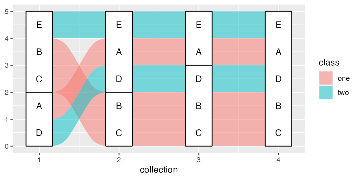
Warning: In addition to parameters like
reverse, when aesthetic variables are prioritized at
all, overlaid alluvial layers must include the same aesthetics in the
same order. (This can produce warnings when the aesthetics are not
recognized by the geom.) Try removing fill = class from the
text geom above to see the risk posed by neglecting this check.
Rather than ordering lodes within, the flow
stat separately orders the flows into and out from,
each stratum. (This precludes a corresponding "alluvia"
option for aes.bind.) By default, the flows are ordered
with respect first to the orders of the strata at the present axis and
second to those at the adjacent axis. Setting aes.bind to
the non-default option "flows" tells
stat_flow() to prioritize flow aesthetics after the strata
of the index axis but before the strata of the adjacent axis:
ggplot(toy, aes(x = collection, stratum = category, alluvium = subject)) +
  stat_flow(aes(fill = class, label = subject), aes.bind = "flows") +
  stat_stratum() +
  stat_flow(geom = "text",
            aes(fill = class, label = subject,
                hjust = after_stat(flow) == "to"),
            aes.bind = "flows")
## Warning in stat_flow(aes(fill = class, label = subject), aes.bind = "flows"):
## Ignoring unknown aesthetics: label## Warning in stat_flow(geom = "text", aes(fill = class, label = subject, hjust =
## after_stat(flow) == : Ignoring unknown aesthetics: fill
Note: The aes.flow parameter tells
geom_flow() how flows should inherit differentiation
aesthetics from adjacent axes—"forward" or
"backward". It does not influence their
positions.
Manual lode ordering
Finally, one may wish to put the lodes at each axis in a predefined
order, subject to their being located in the correct strata. This can be
done by passing a data column to the order aesthetic. For
the toy example, we can pass a vector that puts the cases in the order
of their IDs in the data at every axis:
lode_ord <- rep(seq(5), times = 4)
ggplot(toy, aes(x = collection, stratum = category, alluvium = subject)) +
  stat_alluvium(aes(fill = class, order = lode_ord)) +
  stat_stratum() +
  stat_alluvium(geom = "text",
                aes(fill = class, order = lode_ord, label = subject))
## Warning in stat_alluvium(aes(fill = class, order = lode_ord)): Ignoring
## unknown aesthetics: order## Warning in stat_alluvium(geom = "text", aes(fill = class, order = lode_ord, :
## Ignoring unknown aesthetics: fill and order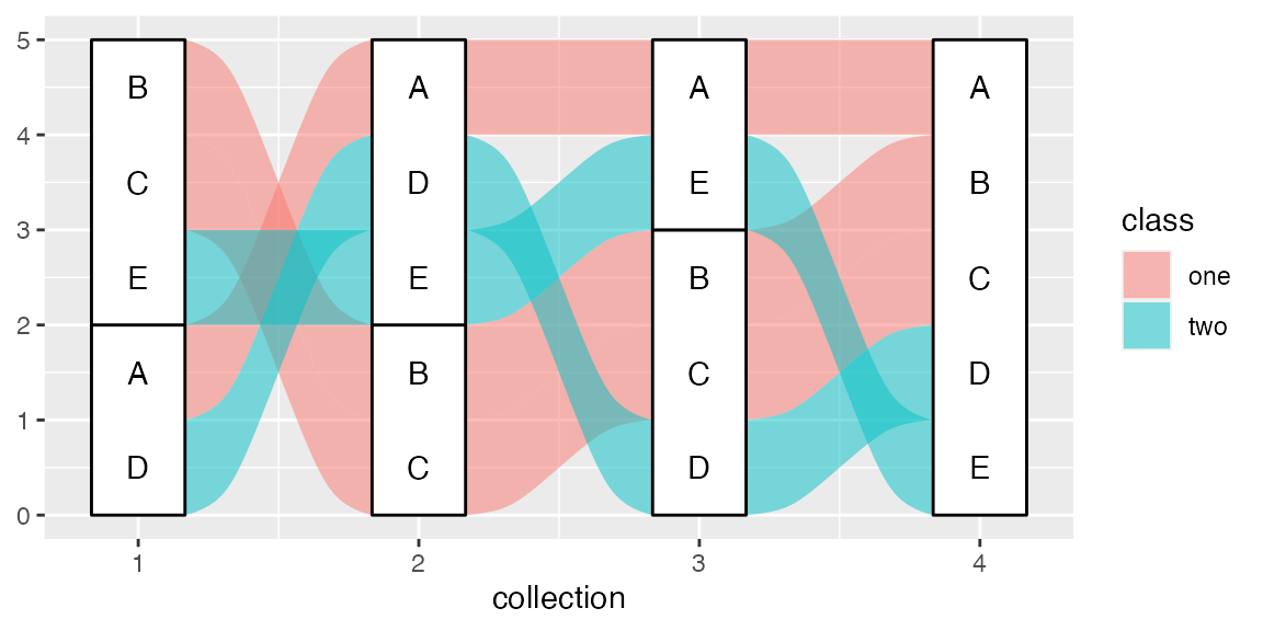
ggplot(toy, aes(x = collection, stratum = category, alluvium = subject)) +
  stat_flow(aes(fill = class, order = lode_ord)) +
  stat_stratum() +
  stat_flow(geom = "text",
            aes(fill = class, order = lode_ord, label = subject,
                hjust = after_stat(flow) == "to"))
## Warning in stat_flow(geom = "text", aes(fill = class, order = lode_ord, :
## Ignoring unknown aesthetics: fill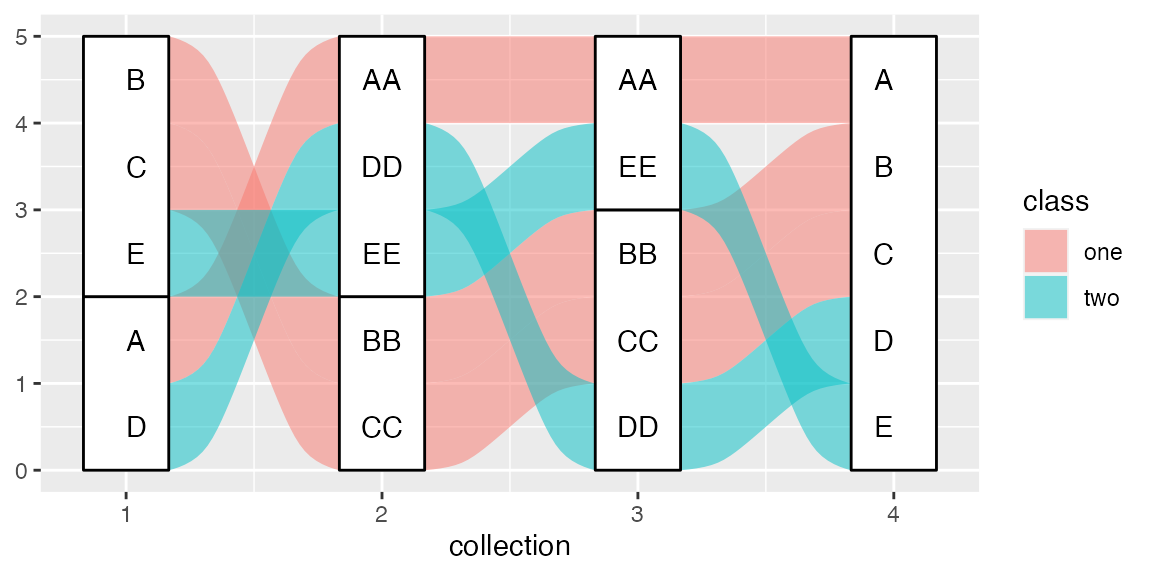
Within each stratum at each axis, the cases are now in order from top to bottom.
Negative strata
In response to an elegant real-world use case, {ggalluvial} can now
handle negative observations in the same way as geom_bar():
by grouping these observations into negative strata and stacking these
strata in the negative y direction (i.e. in the opposite
direction of the positive strata). This new functionality complicates
the above discussion in two ways:
-
Positioning strata: The negative strata could be
reverse-ordered with respect to the positive strata, as in
geom_bar(), or ordered in the same way (vertically, without regard for sign). - Positioning lodes within strata: Two strata may correspond to the same stratum variable at an axis (one positive and one negative), which under-determines the ordering of lodes within strata.
The first issue is binary: Once decreasing and
reverse are chosen, there are only two options for the
negative strata. The choice is made by setting the new
absolute parameter to either TRUE (the
default), which yields a mirror-image ordering, or FALSE,
which adopts the same vertical ordering. This setting also influences
the ordering of lodes within strata at the same nexus as
reverse, namely at the level of the alluvium variable. The
second issue is then handled by creating a deposit variable
with unique values corresponding to each signed stratum
variable value, in the order prescribed by decreasing,
reverse, and absolute. The
deposit variable is then used in place of
stratum for all of the lode-ordering tasks above.
As a point of reference, here is a bar plot of the toy data, with a randomized sign variable used to indicate negative-valued observations:
##    subject collection category class sign
## 1        A          1        Y   one   -1
## 2        B          1        X   one    1
## 3        C          1        X   one    1
## 4        D          1        Y   two   -1
## 5        E          1        X   two    1
## 6        A          2        X   one    1
## 7        B          2        Y   one    1
## 8        C          2        Y   one    1
## 9        D          2        X   two   -1
## 10       E          2        X   two   -1
## 11       A          3        X   one    1
## 12       B          3        Y   one   -1
## 13       C          3        Y   one   -1
## 14       D          3        Y   two    1
## 15       E          3        X   two    1
## 16       A          4        X   one    1
## 17       B          4        X   one    1
## 18       C          4        X   one   -1
## 19       D          4        X   two   -1
## 20       E          4        X   two    1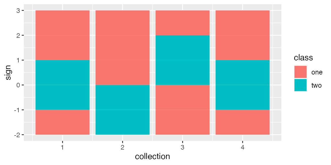
The default behavior, illustrated here with flows, is for the positive strata to proceed downward and the negative strata to proceed upward, in both cases from larger absolute values to zero:
ggplot(toy, aes(x = collection, stratum = category, alluvium = subject,
                y = sign)) +
  geom_flow(aes(fill = class)) +
  geom_stratum() +
  geom_text(stat = "stratum", aes(label = category))
To instead have the strata proceed downward at each axis, and the
lodes downward within each stratum, set absolute = FALSE
(now plotting alluvia):
ggplot(toy, aes(x = collection, stratum = category, alluvium = subject,
                y = sign)) +
  geom_alluvium(aes(fill = class), absolute = FALSE) +
  geom_stratum(absolute = FALSE) +
  geom_text(stat = "alluvium", aes(label = subject), absolute = FALSE)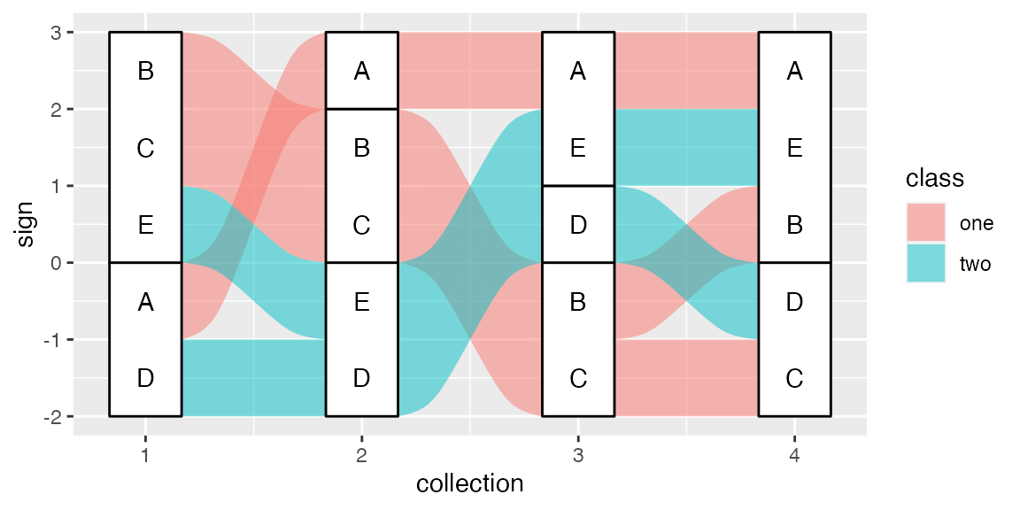
Note again that the labels are consistent with the alluvia and flows,
despite the omission of the fill aesthetic from the text
geom, because the aesthetic variables are not prioritized in the
ordering of the lodes.
More examples
More examples of all of the functionality showcased here can be found
in the documentation for the stat_*() functions, browsable
on the package website.
Appendix
sessioninfo::session_info()## ─ Session info ───────────────────────────────────────────────────────────────
## setting value
## version R version 4.4.2 (2024-10-31)
## os macOS Sonoma 14.4.1
## system aarch64, darwin20
## ui X11
## language en
## collate en_US.UTF-8
## ctype en_US.UTF-8
## tz America/New_York
## date 2025-06-12
## pandoc 2.19 @ /opt/homebrew/bin/ (via rmarkdown)
## quarto NA
##
## ─ Packages ───────────────────────────────────────────────────────────────────
## package * version date (UTC) lib source
## bslib 0.9.0 2025-01-30 [2] CRAN (R 4.4.1)
## cachem 1.1.0 2024-05-16 [2] CRAN (R 4.4.1)
## cli 3.6.5 2025-04-23 [2] CRAN (R 4.4.1)
## desc 1.4.3 2023-12-10 [2] CRAN (R 4.4.1)
## digest 0.6.37 2024-08-19 [2] CRAN (R 4.4.1)
## dplyr 1.1.4 2023-11-17 [2] CRAN (R 4.4.0)
## evaluate 1.0.3 2025-01-10 [2] CRAN (R 4.4.1)
## farver 2.1.2 2024-05-13 [2] CRAN (R 4.4.1)
## fastmap 1.2.0 2024-05-15 [2] CRAN (R 4.4.1)
## fs 1.6.6 2025-04-12 [2] CRAN (R 4.4.1)
## generics 0.1.4 2025-05-09 [2] CRAN (R 4.4.1)
## ggalluvial * 0.12.5 2025-06-12 [1] local
## ggplot2 * 3.5.2 2025-04-09 [2] CRAN (R 4.4.1)
## glue 1.8.0 2024-09-30 [2] CRAN (R 4.4.1)
## gtable 0.3.6 2024-10-25 [2] CRAN (R 4.4.1)
## htmltools 0.5.8.1 2024-04-04 [2] CRAN (R 4.4.1)
## htmlwidgets 1.6.4 2023-12-06 [2] CRAN (R 4.4.0)
## jquerylib 0.1.4 2021-04-26 [2] CRAN (R 4.4.0)
## jsonlite 2.0.0 2025-03-27 [2] CRAN (R 4.4.1)
## knitr 1.50 2025-03-16 [2] CRAN (R 4.4.1)
## labeling 0.4.3 2023-08-29 [2] CRAN (R 4.4.1)
## lifecycle 1.0.4 2023-11-07 [2] CRAN (R 4.4.1)
## magrittr 2.0.3 2022-03-30 [2] CRAN (R 4.4.1)
## pillar 1.10.2 2025-04-05 [2] CRAN (R 4.4.1)
## pkgconfig 2.0.3 2019-09-22 [2] CRAN (R 4.4.1)
## pkgdown 2.1.2 2025-04-28 [2] CRAN (R 4.4.1)
## purrr 1.0.4 2025-02-05 [2] CRAN (R 4.4.1)
## R6 2.6.1 2025-02-15 [2] CRAN (R 4.4.1)
## ragg 1.4.0 2025-04-10 [2] CRAN (R 4.4.1)
## RColorBrewer 1.1-3 2022-04-03 [2] CRAN (R 4.4.1)
## rlang 1.1.6 2025-04-11 [2] CRAN (R 4.4.1)
## rmarkdown 2.29 2024-11-04 [2] CRAN (R 4.4.1)
## sass 0.4.10 2025-04-11 [2] CRAN (R 4.4.1)
## scales 1.4.0 2025-04-24 [2] CRAN (R 4.4.1)
## sessioninfo 1.2.3 2025-02-05 [2] CRAN (R 4.4.1)
## systemfonts 1.2.3 2025-04-30 [2] CRAN (R 4.4.1)
## textshaping 1.0.1 2025-05-01 [2] CRAN (R 4.4.1)
## tibble 3.2.1 2023-03-20 [2] CRAN (R 4.4.0)
## tidyr 1.3.1 2024-01-24 [2] CRAN (R 4.4.1)
## tidyselect 1.2.1 2024-03-11 [2] CRAN (R 4.4.0)
## vctrs 0.6.5 2023-12-01 [2] CRAN (R 4.4.0)
## withr 3.0.2 2024-10-28 [2] CRAN (R 4.4.1)
## xfun 0.52 2025-04-02 [2] CRAN (R 4.4.1)
## yaml 2.3.10 2024-07-26 [2] CRAN (R 4.4.1)
##
## [1] /private/var/folders/4p/3cy0qmp15x9216qsqhh84kzm0000gn/T/Rtmpys5FaI/temp_libpath178905dc69195
## [2] /Library/Frameworks/R.framework/Versions/4.4-arm64/Resources/library
## * ── Packages attached to the search path.
##
## ──────────────────────────────────────────────────────────────────────────────