Alluvial Plots in ggplot2

The {ggalluvial} package is a {ggplot2} extension for producing alluvial plots in a {tidyverse} framework. The design and functionality were originally inspired by the {alluvial} package and have benefitted from the feedback of many users. This vignette

defines the essential components of alluvial plots as used in the naming schemes and documentation (axis, alluvium, stratum, lode, flow),
describes the alluvial data structures recognized by {ggalluvial},
illustrates the new stats and geoms, and
showcases some popular variants on the theme and how to produce them.

Unlike most alluvial and related diagrams, the plots produced by {ggalluvial} are uniquely determined by the data set and statistical transformation. The distinction is detailed in this blog post.

Many other resources exist for visualizing categorical data in R, including several more basic plot types that are likely to more accurately convey proportions to viewers when the data are not so structured as to warrant an alluvial plot. In particular, check out Michael Friendly’s {vcd} and {vcdExtra} packages for a variety of statistically-motivated categorical data visualization techniques, Hadley Wickham’s {productplots} package and Haley Jeppson and Heike Hofmann’s descendant {ggmosaic} package for product or mosaic plots, and Nicholas Hamilton’s {ggtern} package for ternary coordinates. Other related packages are mentioned below.

Alluvial plots

Here’s a quintessential alluvial plot:

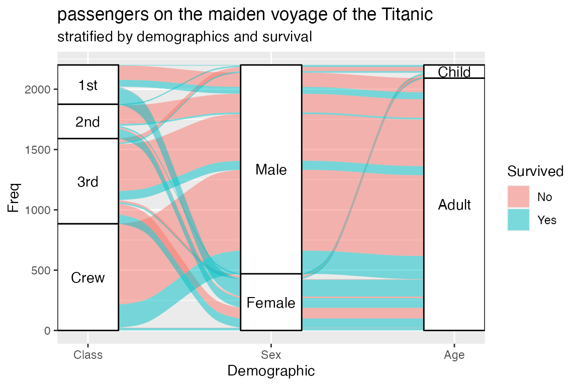
The next section details how the elements of this image encode information about the underlying dataset. For now, we use the image as a point of reference to define the following elements of a typical alluvial plot:

An axis is a dimension (variable) along which the data are vertically arranged at a fixed horizontal position. The plot above uses three categorical axes: Class, Sex, and Age.
The groups at each axis are depicted as opaque blocks called strata. For example, the Class axis contains four strata: 1st, 2nd, 3rd, and Crew.
Horizontal (x-) splines called alluvia span the width of the plot. In this plot, each alluvium corresponds to a fixed value of each axis variable, indicated by its vertical position at the axis, as well as of the Survived variable, indicated by its fill color.
The segments of the alluvia between pairs of adjacent axes are flows.
The alluvia intersect the strata at lodes. The lodes are not visualized in the above plot, but they can be inferred as filled rectangles extending the flows through the strata at each end of the plot or connecting the flows on either side of the center stratum.

As the examples in the next section will demonstrate, which of these elements are incorporated into an alluvial plot depends on both how the underlying data is structured and what the creator wants the plot to communicate.

Alluvial data

{ggalluvial} recognizes two formats of “alluvial data”, treated in detail in the following subsections, but which basically correspond to the “wide” and “long” formats of categorical repeated measures data. A third, tabular (or array), form is popular for storing data with multiple categorical dimensions, such as the Titanic and UCBAdmissions datasets.¹ For consistency with tidy data principles and {ggplot2} conventions, {ggalluvial} does not accept tabular input; base::as.data.frame() converts such an array to an acceptable data frame.

Alluvia (wide) format

The wide format reflects the visual arrangement of an alluvial plot, but “untwisted”: Each row corresponds to a cohort of observations that take a specific value at each variable, and each variable has its own column. An additional column contains the quantity of each row, e.g. the number of observational units in the cohort, which may be used to control the heights of the strata.² Basically, the wide format consists of one row per alluvium. This is the format into which the base function as.data.frame() transforms a frequency table, for instance the 3-dimensional UCBAdmissions dataset:

head(as.data.frame(UCBAdmissions), n = 12)

##       Admit Gender Dept Freq
## 1  Admitted   Male    A  512
## 2  Rejected   Male    A  313
## 3  Admitted Female    A   89
## 4  Rejected Female    A   19
## 5  Admitted   Male    B  353
## 6  Rejected   Male    B  207
## 7  Admitted Female    B   17
## 8  Rejected Female    B    8
## 9  Admitted   Male    C  120
## 10 Rejected   Male    C  205
## 11 Admitted Female    C  202
## 12 Rejected Female    C  391

is_alluvia_form(as.data.frame(UCBAdmissions), axes = 1:3, silent = TRUE)

## [1] TRUE

This format is inherited from the first release of {ggalluvial}, which modeled it after usage in {alluvial}: The user declares any number of axis variables, which stat_alluvium() and stat_stratum() recognize and process in a consistent way:³

ggplot(as.data.frame(UCBAdmissions),
       aes(y = Freq, axis1 = Gender, axis2 = Dept)) +
  geom_alluvium(aes(fill = Admit), width = 1/12) +
  geom_stratum(width = 1/12, fill = "black", color = "grey") +
  geom_label(stat = "stratum", aes(label = after_stat(stratum))) +
  scale_x_discrete(limits = c("Gender", "Dept"), expand = c(.05, .05)) +
  scale_fill_brewer(type = "qual", palette = "Set1") +
  ggtitle("UC Berkeley admissions and rejections, by sex and department")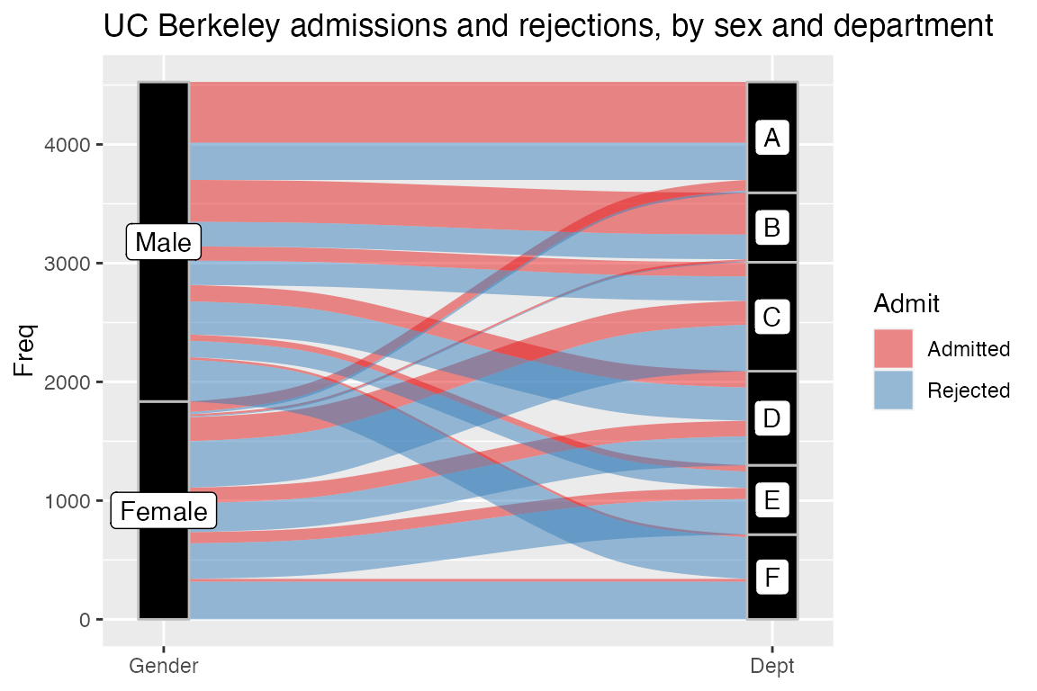

An important feature of these plots is the meaningfulness of the vertical axis: No gaps are inserted between the strata, so the total height of the plot reflects the cumulative quantity of the observations. The plots produced by {ggalluvial} conform (somewhat; keep reading) to the “grammar of graphics” principles of {ggplot2}, and this prevents users from producing “free-floating” visualizations like the Sankey diagrams showcased here.⁴ {ggalluvial} parameters and native {ggplot2} functionality can also produce parallel sets plots, illustrated here using the HairEyeColor dataset:⁵ ⁶

ggplot(as.data.frame(HairEyeColor),
       aes(y = Freq,
           axis1 = Hair, axis2 = Eye, axis3 = Sex)) +
  geom_alluvium(aes(fill = Eye),
                width = 1/8, knot.pos = 0, reverse = FALSE) +
  scale_fill_manual(values = c(Brown = "#70493D", Hazel = "#E2AC76",
                               Green = "#3F752B", Blue = "#81B0E4")) +
  guides(fill = "none") +
  geom_stratum(alpha = .25, width = 1/8, reverse = FALSE) +
  geom_text(stat = "stratum", aes(label = after_stat(stratum)),
            reverse = FALSE) +
  scale_x_continuous(breaks = 1:3, labels = c("Hair", "Eye", "Sex")) +
  coord_flip() +
  ggtitle("Eye colors of 592 subjects, by sex and hair color")

## Warning in to_lodes_form(data = data, axes = axis_ind, discern =
## params$discern): Some strata appear at multiple axes.
## Warning in to_lodes_form(data = data, axes = axis_ind, discern =
## params$discern): Some strata appear at multiple axes.
## Warning in to_lodes_form(data = data, axes = axis_ind, discern =
## params$discern): Some strata appear at multiple axes.

(The warning is due to the “Hair” and “Eye” axes having the value “Brown” in common.)

This format and functionality are useful for many applications and will be retained in future versions. They also involve some conspicuous deviations from {ggplot2} norms:

The axis[0-9]* position aesthetics are non-standard: they are not an explicit set of parameters but a family based on a regular expression pattern; and at least one, but no specific one, is required.
stat_alluvium() ignores any argument to the group aesthetic; instead, StatAlluvium$compute_panel() uses group to link the rows of the internally-transformed dataset that correspond to the same alluvium.
The horizontal axis must be manually corrected (using scale_x_discrete() or scale_x_continuous()) to reflect the implicit categorical variable identifying the axis.

Furthermore, format aesthetics like fill are necessarily fixed for each alluvium; they cannot, for example, change from axis to axis according to the value taken at each. This means that, although they can reproduce the branching-tree structure of parallel sets, this format cannot be used to produce alluvial plots with color schemes such as those featured here (“Controlling colors”), which are “reset” at each axis.

Note also that the stratum variable produced by stat_stratum() (called by geom_text()) is computed during the statistical transformation and must be recovered using after_stat() as a calculated aesthetic.

Lodes (long) format

The long format recognized by {ggalluvial} contains one row per lode, and can be understood as the result of “gathering” (in a deprecated {dplyr} sense) or “pivoting” (in the Microsoft Excel or current {dplyr} sense) the axis columns of a dataset in the alluvia format into a key-value pair of columns encoding the axis as the key and the stratum as the value. This format requires an additional indexing column that links the rows corresponding to a common cohort, i.e. the lodes of a single alluvium:

UCB_lodes <- to_lodes_form(as.data.frame(UCBAdmissions),
                           axes = 1:3,
                           id = "Cohort")
head(UCB_lodes, n = 12)

##    Freq Cohort     x  stratum
## 1   512      1 Admit Admitted
## 2   313      2 Admit Rejected
## 3    89      3 Admit Admitted
## 4    19      4 Admit Rejected
## 5   353      5 Admit Admitted
## 6   207      6 Admit Rejected
## 7    17      7 Admit Admitted
## 8     8      8 Admit Rejected
## 9   120      9 Admit Admitted
## 10  205     10 Admit Rejected
## 11  202     11 Admit Admitted
## 12  391     12 Admit Rejected

is_lodes_form(UCB_lodes, key = x, value = stratum, id = Cohort, silent = TRUE)

## [1] TRUE

The functions that convert data between wide (alluvia) and long (lodes) format include several parameters that help preserve ancillary information. See help("alluvial-data") for examples.

The same stat and geom can receive data in this format using a different set of positional aesthetics, also specific to {ggalluvial}:

x, the “key” variable indicating the axis to which the row corresponds, which are to be arranged along the horizontal axis;
stratum, the “value” taken by the axis variable indicated by x; and
alluvium, the indexing scheme that links the rows of a single alluvium.

Heights can vary from axis to axis, allowing users to produce bump charts like those showcased here.⁷ In these cases, the strata contain no more information than the alluvia and often are not plotted. For convenience, both stat_alluvium() and stat_flow() will accept arguments for x and alluvium even if none is given for stratum.⁸ As an example, we can group countries in the Refugees dataset by region, in order to compare refugee volumes at different scales:

data(Refugees, package = "alluvial")
country_regions <- c(
  Afghanistan = "Middle East",
  Burundi = "Central Africa",
  `Congo DRC` = "Central Africa",
  Iraq = "Middle East",
  Myanmar = "Southeast Asia",
  Palestine = "Middle East",
  Somalia = "Horn of Africa",
  Sudan = "Central Africa",
  Syria = "Middle East",
  Vietnam = "Southeast Asia"
)
Refugees$region <- country_regions[Refugees$country]
ggplot(data = Refugees,
       aes(x = year, y = refugees, alluvium = country)) +
  geom_alluvium(aes(fill = country, colour = country),
                alpha = .75, decreasing = FALSE, outline.type = "upper") +
  scale_x_continuous(breaks = seq(2003, 2013, 2)) +
  theme_bw() +
  theme(axis.text.x = element_text(angle = -30, hjust = 0)) +
  scale_fill_brewer(type = "qual", palette = "Set3") +
  scale_color_brewer(type = "qual", palette = "Set3") +
  facet_wrap(~ region, scales = "fixed") +
  ggtitle("refugee volume by country and region of origin")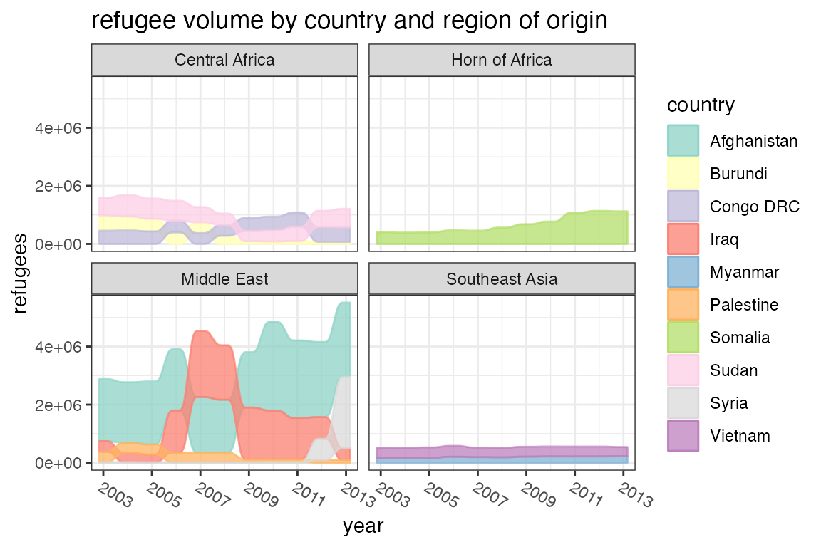

The format allows us to assign aesthetics that change from axis to axis along the same alluvium, which is useful for repeated measures datasets. This requires generating a separate graphical object for each flow, as implemented in geom_flow(). The plot below uses a set of (changes to) students’ academic curricula over the course of several semesters. Since geom_flow() calls stat_flow() by default (see the next example), we override it with stat_alluvium() in order to track each student across all semesters:

data(majors)
majors$curriculum <- as.factor(majors$curriculum)
ggplot(majors,
       aes(x = semester, stratum = curriculum, alluvium = student,
           fill = curriculum, label = curriculum)) +
  scale_fill_brewer(type = "qual", palette = "Set2") +
  geom_flow(stat = "alluvium", lode.guidance = "frontback",
            color = "darkgray") +
  geom_stratum() +
  theme(legend.position = "bottom") +
  ggtitle("student curricula across several semesters")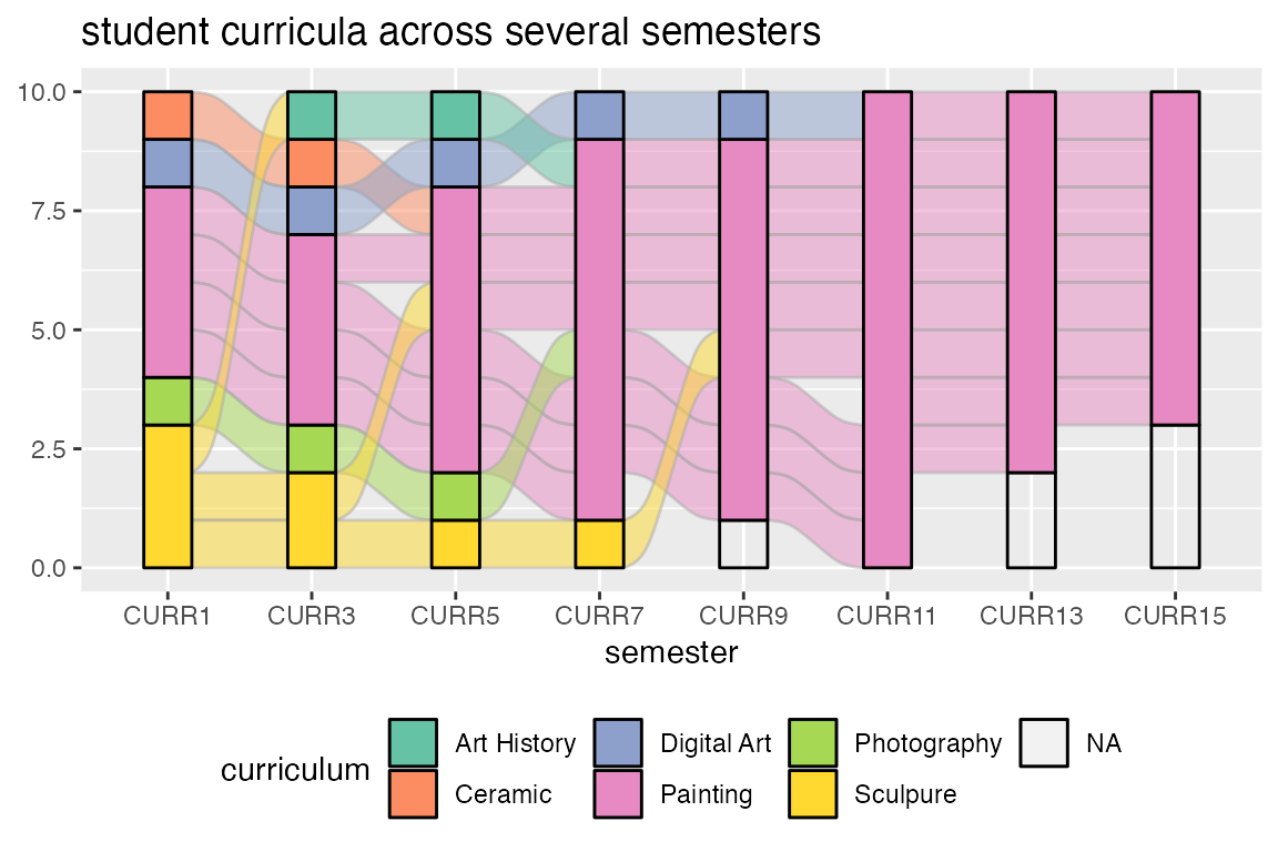

The stratum heights y are unspecified, so each row is given unit height. This example demonstrates one way {ggalluvial} handles missing data. The alternative is to set the parameter na.rm to TRUE.⁹ Missing data handling (specifically, the order of the strata) also depends on whether the stratum variable is character or factor/numeric.

Finally, lode format gives us the option to aggregate the flows between adjacent axes, which may be appropriate when the transitions between adjacent axes are of primary importance. We can demonstrate this option on data from the influenza vaccination surveys conducted by the RAND American Life Panel. The data, including one question from each of three surveys, has been aggregated by response profile: Each “subject” (mapped to alluvium) actually represents a cohort of subjects who responded the same way on all three questions, and the size of each cohort (mapped to y) is recorded in “freq”.

data(vaccinations)
vaccinations <- transform(vaccinations,
                          response = factor(response, rev(levels(response))))
ggplot(vaccinations,
       aes(x = survey, stratum = response, alluvium = subject,
           y = freq,
           fill = response, label = response)) +
  scale_x_discrete(expand = c(.1, .1)) +
  geom_flow() +
  geom_stratum(alpha = .5) +
  geom_text(stat = "stratum", size = 3) +
  theme(legend.position = "none") +
  ggtitle("vaccination survey responses at three points in time")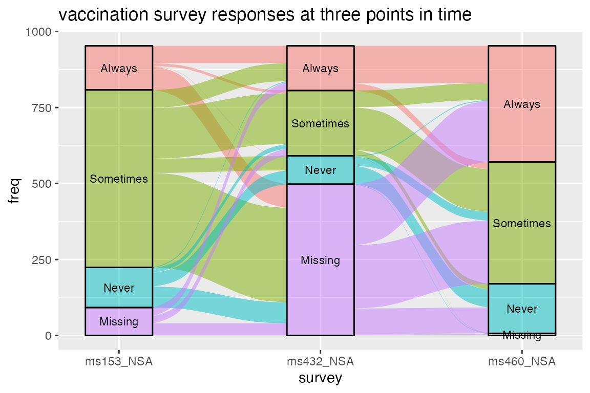

This plot ignores any continuity between the flows between axes. This “memoryless” statistical transformation yields a less cluttered plot, in which at most one flow proceeds from each stratum at one axis to each stratum at the next, but at the cost of being able to track each cohort across the entire plot.

Appendix

sessioninfo::session_info()

## ─ Session info ───────────────────────────────────────────────────────────────
##  setting  value
##  version  R version 4.4.2 (2024-10-31)
##  os       macOS Sonoma 14.4.1
##  system   aarch64, darwin20
##  ui       X11
##  language en
##  collate  en_US.UTF-8
##  ctype    en_US.UTF-8
##  tz       America/New_York
##  date     2025-06-12
##  pandoc   2.19 @ /opt/homebrew/bin/ (via rmarkdown)
##  quarto   NA
## 
## ─ Packages ───────────────────────────────────────────────────────────────────
##  package      * version date (UTC) lib source
##  bslib          0.9.0   2025-01-30 [2] CRAN (R 4.4.1)
##  cachem         1.1.0   2024-05-16 [2] CRAN (R 4.4.1)
##  cli            3.6.5   2025-04-23 [2] CRAN (R 4.4.1)
##  desc           1.4.3   2023-12-10 [2] CRAN (R 4.4.1)
##  digest         0.6.37  2024-08-19 [2] CRAN (R 4.4.1)
##  dplyr          1.1.4   2023-11-17 [2] CRAN (R 4.4.0)
##  evaluate       1.0.3   2025-01-10 [2] CRAN (R 4.4.1)
##  farver         2.1.2   2024-05-13 [2] CRAN (R 4.4.1)
##  fastmap        1.2.0   2024-05-15 [2] CRAN (R 4.4.1)
##  fs             1.6.6   2025-04-12 [2] CRAN (R 4.4.1)
##  generics       0.1.4   2025-05-09 [2] CRAN (R 4.4.1)
##  ggalluvial   * 0.12.5  2025-06-12 [1] local
##  ggplot2      * 3.5.2   2025-04-09 [2] CRAN (R 4.4.1)
##  glue           1.8.0   2024-09-30 [2] CRAN (R 4.4.1)
##  gtable         0.3.6   2024-10-25 [2] CRAN (R 4.4.1)
##  htmltools      0.5.8.1 2024-04-04 [2] CRAN (R 4.4.1)
##  htmlwidgets    1.6.4   2023-12-06 [2] CRAN (R 4.4.0)
##  jquerylib      0.1.4   2021-04-26 [2] CRAN (R 4.4.0)
##  jsonlite       2.0.0   2025-03-27 [2] CRAN (R 4.4.1)
##  knitr          1.50    2025-03-16 [2] CRAN (R 4.4.1)
##  labeling       0.4.3   2023-08-29 [2] CRAN (R 4.4.1)
##  lifecycle      1.0.4   2023-11-07 [2] CRAN (R 4.4.1)
##  magrittr       2.0.3   2022-03-30 [2] CRAN (R 4.4.1)
##  pillar         1.10.2  2025-04-05 [2] CRAN (R 4.4.1)
##  pkgconfig      2.0.3   2019-09-22 [2] CRAN (R 4.4.1)
##  pkgdown        2.1.2   2025-04-28 [2] CRAN (R 4.4.1)
##  purrr          1.0.4   2025-02-05 [2] CRAN (R 4.4.1)
##  R6             2.6.1   2025-02-15 [2] CRAN (R 4.4.1)
##  ragg           1.4.0   2025-04-10 [2] CRAN (R 4.4.1)
##  RColorBrewer   1.1-3   2022-04-03 [2] CRAN (R 4.4.1)
##  rlang          1.1.6   2025-04-11 [2] CRAN (R 4.4.1)
##  rmarkdown      2.29    2024-11-04 [2] CRAN (R 4.4.1)
##  sass           0.4.10  2025-04-11 [2] CRAN (R 4.4.1)
##  scales         1.4.0   2025-04-24 [2] CRAN (R 4.4.1)
##  sessioninfo    1.2.3   2025-02-05 [2] CRAN (R 4.4.1)
##  systemfonts    1.2.3   2025-04-30 [2] CRAN (R 4.4.1)
##  textshaping    1.0.1   2025-05-01 [2] CRAN (R 4.4.1)
##  tibble         3.2.1   2023-03-20 [2] CRAN (R 4.4.0)
##  tidyr          1.3.1   2024-01-24 [2] CRAN (R 4.4.1)
##  tidyselect     1.2.1   2024-03-11 [2] CRAN (R 4.4.0)
##  vctrs          0.6.5   2023-12-01 [2] CRAN (R 4.4.0)
##  withr          3.0.2   2024-10-28 [2] CRAN (R 4.4.1)
##  xfun           0.52    2025-04-02 [2] CRAN (R 4.4.1)
##  yaml           2.3.10  2024-07-26 [2] CRAN (R 4.4.1)
## 
##  [1] /private/var/folders/4p/3cy0qmp15x9216qsqhh84kzm0000gn/T/Rtmpys5FaI/temp_libpath178905dc69195
##  [2] /Library/Frameworks/R.framework/Versions/4.4-arm64/Resources/library
##  * ── Packages attached to the search path.
## 
## ──────────────────────────────────────────────────────────────────────────────

Jason Cory Brunson

2025-06-12

Alluvial plots

Alluvial data

Alluvia (wide) format

Lodes (long) format

Appendix