| tags:books polyamory web scraping principal components analysis biplot categories:curiosity
the dimensions of (abstracted) polyamory literature
I’ve gained immensely from reading the handful of non-fiction books on polyamory i’ve made time to, including Dossie Easton and Janet Hardy’s The Ethical Slut and Franklin Veaux and Eve Rickert’s More Than Two. While i’ve identified as poly since i discovered the term in grad school, i exhibit at least my share of emotional immaturity, and in addition to actual experience building healthy relationships i know i’d benefit from funneling a bit more of this literature into my reading queue. So, with a small group of friends (which has reduced for the time being to someone i’m dating plus myself), i recently started a poly/kink book club.
From the start, i intended to slide fiction, fantasy/scifi, memoir, anthropology, history, and any other genres i could discover onto our shelf, to accrue a well-rounded appreciation for what was available. Though this of course put me to wondering how i could even learn the contours of the poly literature, in order to ensure that i sampled widely from it! Fortunes of timing provided me with three excellent resources:
- a Goodreads account;
- a blog tutorial by Mara Averick on using R packages to scrape and crunch Goodreads data; and
- a book by Julia Silge and David Robinson on doing text mining in tidyverse style.
The tutorial and its sequel will get you up to speed; i’ll outline my web-scraping script and focus mostly on the analysis.
scrape
It would be, let’s say, impractical to manually search out books with explicitly poly content or themes, and even then i’d likely miss a bunch whose descriptions don’t let on too clearly. Fortunately, Goodreads allows users both to curate thematic lists and to tag their lists with keywords! Here is the collection of lists tagged “polyamory”, numbering in the dozens. Helpfully, the lists span genres, including fiction, young adult, memoirs, specific configurations like triads, and space opera (natch). Less helpfully, they also range more broadly in topic and theme, for example exotica, sex positivity, and love. On the whole, though, the tag seems like a good candidate for a one-off look.
There are other relevant tags, of course, like “open-relationships”. But the others i’ve found turn out to be far less sensitive and often less specific. For example, “nonmonogamy” turns up two relevant lists but “non monogamy” turns up a third, and “swinging” yields four lists, of which one is a conspicuous false positive. For simplicity, i’ll stick with the “polyamory” tag. This is something i can revisit if the results aren’t facially relevant.
My code (in the supplementary folder) scrapes first the list URLs from the meta-list (polyamory_listopia), then the book URLs from each list page (polyamory_lists), and finally metadata from each book page (polyamory_books): title, link, author(s), genre(s), and book description. While the authors and title serve as identifiers and the genres may serve as annotations, the descriptions constitute the raw material on which i’ll perform a text analysis. (The full texts of the books themselves are not so freely available,1 the titles are unlikely to reliably encode recurring features, and the genres are likely too few to discriminate except between broad categories.)
It’s important to note that there are two tiers of redundancy in the book list, only one of which i eliminate. First, the same Goodreads entry2 may appear in multiple lists; second, the same book may have been erroneously entered into Goodreads multiple times (which may appear in different lists or even the same list). It would require a few hours of manual curation to resolve the latter problem,3 and i haven’t put in that time here; but the first problem is easily handled using group_by() and summarize().
crunch
Here is the book list obtained from the scraping script, slightly tidied, using the identifying string of the URL as a unique identifier:
library(tidyverse)
read_rds(here::here("supplementary/goodreads-polyamory-booklist.rds")) %>%
  ungroup() %>%
  select(title = title_page, id = link, lists, genres, description) %>%
  mutate(short_title = str_replace(title, "(: .+$)|( \\(.+$)", "")) %>%
  mutate(id = str_replace(id, "/book/show/([0-9]+)[^0-9].*$", "\\1")) %>%
  mutate(id = as.integer(id)) %>%
  print() -> polyamory_booklist
## # A tibble: 1,179 x 6
## title id lists genres description short_title
## <chr> <int> <chr> <chr> <chr> <chr>
## 1 100 Love … 1.13e4 Books on … Poetry|Cla… Against the ba… 100 Love Sonn…
## 2 199 Ways … 1.61e7 Sex, Love… "" 199 Ways To Im… 199 Ways To I…
## 3 30th Cent… 3.53e7 Ménage Po… Science Fi… CAPTAIN JENNIF… 30th Century
## 4 A + E 4ev… 1.24e7 The Most … Sequential… Asher Machnik … A + E 4ever
## 5 A Bear's … 2.73e7 Ménage Po… Erotica|Me… Most days, Oli… A Bear's Jour…
## 6 A Bear's … 4.06e7 Polyfi Tr… Paranormal… Most days, Oli… A Bear's Jour…
## 7 A Bear's … 2.71e7 Ménage Po… Erotica|Me… Charlotte “Cha… A Bear's Mercy
## 8 A Bear's … 4.06e7 Polyfi Tr… Menage|M M… Charlotte “Cha… A Bear's Mercy
## 9 A Bear's … 2.68e7 Ménage Po… Erotica|Me… Quinn Taylor h… A Bear's Neme…
## 10 A Bear's … 4.05e7 Polyfi Tr… Fantasy|Pa… Quinn Taylor h… A Bear's Neme…
## # … with 1,169 more rows(Some of the duplicate entries are evident.) My goal here is to represent these 1,179 book entries as points (or vectors) in some low-dimensional space, based on the co-occurrence of words in their descriptions. Ideally, the coordinate dimenisons of this space will correspond to identifiable features that will help characterize the dimensions and allow the dimensions to characterize individual books in turn. If the number of dimensions is low enough, then it will also be possible to visualize the point cloud and coordinate vectors.
word counts
Adapting a workflow from the tidytext book, i first “unnest” the book list—in the tidyr sense, except using a tidytext method specific to strings of written language. “Stop” words are articles, prepositions, and other words that add little to no value to a text analysis; instances of them in the unnested data are excluded via an anti-join. Finally, i count the number of times each word is used in each description as a new variable \(n\).
library(tidytext)
polyamory_booklist %>%
  mutate(clean_descr = str_replace_all(description, "[^[:alpha:]\\s]", " ")) %>%
  mutate(clean_descr = str_trim(clean_descr)) %>%
  select(-description) %>%
  unnest_tokens(word, clean_descr) %>%
  anti_join(stop_words, by = "word") %>%
  count(title, short_title, id, lists, genres, word, name = "n") %>%
  print() -> polybooks_wordcounts
## # A tibble: 76,194 x 7
## title short_title id lists genres word n
## <chr> <chr> <int> <chr> <chr> <chr> <int>
## 1 100 Love S… 100 Love Sonn… 11339 Books on… Poetry|Classi… backdrop 1
## 2 100 Love S… 100 Love Sonn… 11339 Books on… Poetry|Classi… beloved 1
## 3 100 Love S… 100 Love Sonn… 11339 Books on… Poetry|Classi… celebra… 1
## 4 100 Love S… 100 Love Sonn… 11339 Books on… Poetry|Classi… de 1
## 5 100 Love S… 100 Love Sonn… 11339 Books on… Poetry|Classi… delicate 1
## 6 100 Love S… 100 Love Sonn… 11339 Books on… Poetry|Classi… flowers 1
## 7 100 Love S… 100 Love Sonn… 11339 Books on… Poetry|Classi… hot 1
## 8 100 Love S… 100 Love Sonn… 11339 Books on… Poetry|Classi… isla 1
## 9 100 Love S… 100 Love Sonn… 11339 Books on… Poetry|Classi… love 2
## 10 100 Love S… 100 Love Sonn… 11339 Books on… Poetry|Classi… matilde 1
## # … with 76,184 more rowsA couple more word counts that will be useful downstream are the number \(d\) of book descriptions that use each word and the total number \(m\) of uses across the corpus.
polybooks_wordcounts %>%
  left_join(
    polybooks_wordcounts %>%
      group_by(word) %>%
      summarize(d = n(), m = sum(n)),
    by = c("word")
  ) %>%
  filter(m >= 12) %>%
  arrange(desc(d), desc(n)) %>%
  print() -> polybooks_wordusages
## # A tibble: 48,020 x 9
## title short_title id lists genres word n d m
## <chr> <chr> <int> <chr> <chr> <chr> <int> <int> <int>
## 1 What Love… What Love Is 2.95e7 Best … Nonfictio… love 16 495 1226
## 2 The Four … The Four Lo… 3.06e4 Books… Christian… love 14 495 1226
## 3 The Futur… The Future … 7.21e5 Books… Relations… love 14 495 1226
## 4 Why We Lo… Why We Love 1.32e5 Sex, … Psycholog… love 14 495 1226
## 5 Longing f… Longing for… 1.73e7 Sex, … "" love 13 495 1226
## 6 The Art o… The Art of … 1.41e4 Books… Psycholog… love 13 495 1226
## 7 Rogue Eve… Rogue Ever … 4.52e7 FFF+ … Romance|C… love 12 495 1226
## 8 Ardently:… Ardently 2.56e7 Books… Classics|… love 11 495 1226
## 9 Love Magi… Love Magic 1.36e7 Sex, … "" love 10 495 1226
## 10 In Praise… In Praise o… 1.36e7 Books… Philosoph… love 9 495 1226
## # … with 48,010 more rows2,197 distinct words appear in these descriptions (omitting the stop words). Happily, the most prevalent (and, it turns out, most frequent) word in these descriptions is “love”. <83
relative frequencies
Its ubiquity makes “love” unlikely to be an effective token for the purpose of mapping this book collection in coordinate space: If a feature describes everything, then it describes nothing. The traditional usefulness weighting on words is instead the term frequency–inverse document frequency, or tf-idf. This is the product of two quotients: the term frequency \(\frac{n}{N}\) for a given book, where \(N\) is the number of words in its description; and (the logarithm of) the inverse of the document frequency \(\frac{d}{D}\), where \(D\) is the number of books (descriptions) in the corpus. The tidytext package provides a helper function for this step, bind_tf_idf(), which obviates the previous chunk. Additionally i’ve filtered out the less discriminating words (having maximum td-idf at most \(0.1\)):
polybooks_wordcounts %>%
  bind_tf_idf(word, id, n) %>%
  group_by(word) %>% filter(max(tf_idf) > .1) %>% ungroup() %>%
  select(title, short_title, id, lists, genres, word, tf_idf) %>%
  print() -> polybooks_tfidf
## # A tibble: 59,759 x 7
## title short_title id lists genres word tf_idf
## <chr> <chr> <int> <chr> <chr> <chr> <dbl>
## 1 100 Love S… 100 Love Sonn… 11339 Books on… Poetry|Classi… backdr… 0.189
## 2 100 Love S… 100 Love Sonn… 11339 Books on… Poetry|Classi… beloved 0.136
## 3 100 Love S… 100 Love Sonn… 11339 Books on… Poetry|Classi… celebr… 0.171
## 4 100 Love S… 100 Love Sonn… 11339 Books on… Poetry|Classi… de 0.136
## 5 100 Love S… 100 Love Sonn… 11339 Books on… Poetry|Classi… delica… 0.162
## 6 100 Love S… 100 Love Sonn… 11339 Books on… Poetry|Classi… flowers 0.189
## 7 100 Love S… 100 Love Sonn… 11339 Books on… Poetry|Classi… hot 0.0738
## 8 100 Love S… 100 Love Sonn… 11339 Books on… Poetry|Classi… isla 0.212
## 9 100 Love S… 100 Love Sonn… 11339 Books on… Poetry|Classi… love 0.0573
## 10 100 Love S… 100 Love Sonn… 11339 Books on… Poetry|Classi… matilde 0.235
## # … with 59,749 more rowsI’ll use these remaining 9,005 words to make a first pass at gauging the dimensionality of the corpus and visualizing the books and features, using classical PCA. This requires widening the table into a classical data matrix having one row per book, one column per word, and log-transformed tf-idf values (to better mimic normality). The words are capitalized to prevent conflicts with existing column names, and a separate tibble includes only the metadata.
polybooks_tfidf %>%
  mutate(log_tf_idf = log(tf_idf)) %>%
  select(-tf_idf) %>%
  mutate(word = toupper(word)) %>%
  spread(word, log_tf_idf, fill = 0) ->
  polybooks_tfidf_wide
polybooks_tfidf_wide %>%
  select(title, short_title, id, lists, genres) ->
  polybooks_meta
R implementations of ordination methods tend to produce atrociously unreadable output when sample sizes and variable dimensions grow large, so this is an especially apt place to invoke ordr.4 The ID numbers serve as unique identifiers, just in case duplicate entries for the same book have exactly the same title, and so short titles are bound back in after the PCA:
library(ordr)
polybooks_tfidf_wide %>%
  select(-title, -short_title, -lists, -genres) %>%
  column_to_rownames("id") %>%
  as.matrix() %>%
  prcomp() %>%
  as_tbl_ord() %>%
  augment() %>%
  bind_cols_u(select(polybooks_meta, short_title)) %>%
  print() -> polybooks_pca
## # A tbl_ord of class 'prcomp': (1170 x 1170) x (9005 x 1170)'
## # 1170 coordinates: PC1, PC2, ..., PC1170
## #
## # U: [ 1170 x 1170 | 2 ]
## PC1 PC2 PC3 ... | .name short_title
## | <chr> <chr>
## 1 -3.12 0.0527 -0.00351 | 1 11339 100 Love Sonnets
## 2 2.69 -3.08 3.14 ... | 2 161489… 199 Ways To Improve You…
## 3 1.93 1.14 0.819 | 3 352771… 30th Century
## 4 1.52 -0.958 -0.255 | 4 124467… A + E 4ever
## 5 2.71 4.21 -1.04 | 5 272627… A Bear's Journey
## # … with 1,165 more rows
## #
## # V: [ 9005 x 1170 | 2 ]
## PC1 PC2 PC3 ... | .name .center
## | <chr> <dbl>
## 1 0.00340 0.0000956 0.00569 | 1 À -0.0182
## 2 -0.00138 0.00104 -0.000921 ... | 2 AARON -0.00836
## 3 -0.00236 -0.00257 0.00216 | 3 ABANDONED -0.0203
## 4 0.000251 0.0000375 -0.0000183 | 4 ABBEY -0.000521
## 5 0.000370 0.00000365 0.000444 | 5 ABBI -0.00174
## # … with 9,000 more rowsThe ubiquitous scree plot helps gauge the dimensionality of the tf-idf space, though for readability i’m restricting it to the principal components (PCs) that account for at least \(0.4\%\) of the total variance each:
polybooks_pca %>%
  fortify(.matrix = "coord") %>%
  filter(.prop_var > .004) %>%
  ggplot(aes(x = .name, y = .prop_var)) +
  geom_bar(stat = "identity") +
  labs(x = "", y = "Proportion of variance") +
  theme(axis.text.x = element_text(angle = 90))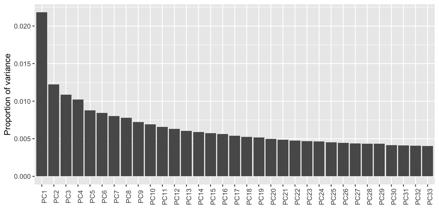
This is not promising: The first PC accounts for less than one fortieth of the total variation, though the remaining PCs are even less distinctive. A 1-dimensional biplot would make the most sense, but in order to add some annotation i’m extending it to 2 dimensions, with the caveat that the second, vertical dimension should be understood—for any specific slice along PC1—as a more or less arbitrary perspective on a more or less spherical cloud. I’ll highlight and label the convex hull of the projected cloud to help think about how the books are dispersed:
ggbiplot(polybooks_pca) +
  geom_u_point(alpha = .5) +
  geom_u_point(stat = "chull", color = "red") +
  geom_u_label_repel(
    stat = "chull", aes(label = short_title),
    color = "red", alpha = .75, size = 3
  ) +
  scale_x_continuous(expand = expand_scale(mult = c(0.4, 0.1)))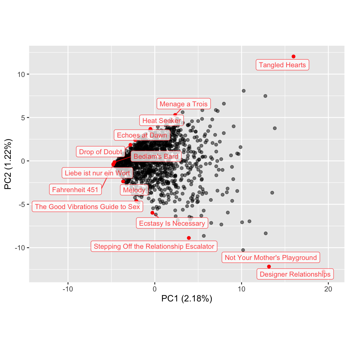
The biplot exhibits a common pattern, with the bulk of observations clumped together in a corner and an increasingly thin periphery pushing conically outward. This pattern tends to emerge when the underlying variables are better understood as features than as spectra: When two distinctive and mutually repulsive (not necessarily to say mutually exclusive) features describe a data set, PCA will tend to yield a boomerang shape along the first two PCs. A classic example of this is a set of clinical and laboratory test data collected by G.M. Reaven and R. Miller for a diabetic cohort, illustrated here by Michael Friendly. When more features are present and remain mutually repulsive, the resulting bouquets tend to project onto PC1 and PC2 as cones. This is in contrast to settings in which the constituent variables are uncorrelated, in which point clouds, whether high-dimensional or projected onto PCs, tend to be spherical (as discussed in a previous post).
It might therefore make more sense to get a reading of the books farthest from the clump, i.e. with the most extreme scores along PC1, rather than those on the outskirts of the point cloud on PC1 and PC2 together.5 To that end, i’ll take the books with the top 12 scores along, and the words with the top 12 loadings onto, PC1:
polybooks_pca %>%
  tidy(.matrix = "both", include = "all") %>%
  select(-starts_with("PC"), PC1, -.center) %>%
  group_by(.matrix) %>%
  arrange(desc(PC1)) %>%
  top_n(12, PC1) %>%
  mutate(name = ifelse(is.na(short_title), tolower(.name), short_title)) %>%
  ggplot(aes(x = reorder(name, PC1), y = PC1)) +
  facet_wrap(~ .matrix, scales = "free") +
  coord_flip() +
  geom_bar(stat = "identity") +
  labs(x = "Score / Loading")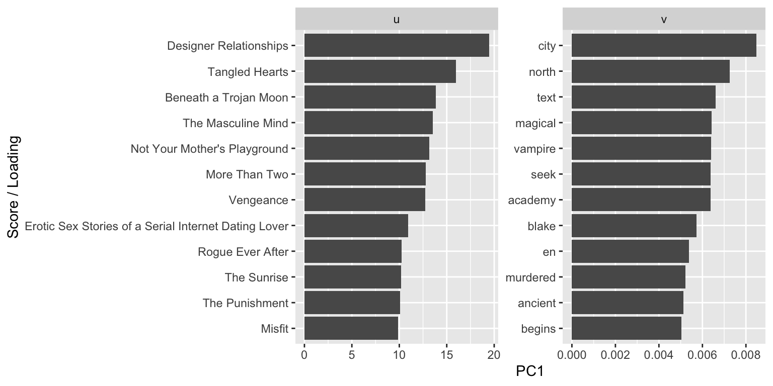
The scores and loadings are likewise not very discriminating, but they are suggestive of the varieties of polyamory or poly-adjacent literature that push up against its boundaries: Many of the titles suggest niche subgenres of fiction, alongside some general advice or lifestyle volumes. Words like “magical”, “vampire”, “murdered”, “ancient”, and, i’d say, even “city” and “begins” are indicative of the former, while “text” and “academy” may be of the latter. Overall, though, this is not a very informative dimension. Rather than separating one genre from others, it’s detecting unique descriptions from a medley of genres. And this is just what one might expect from the conical shape of the point cloud.
So, it seems likely that discriminating features exist along which these descriptions are organized, though principal components—which by definition capture variation, not distinction—aren’t a good tool for detecting them. This is still good news for my ultimate goal of identifying these features. In a follow-up post i’ll use a couple of different tactics, one from text mining and the other not yet widely used.
Though making word frequency data publicly available would presumably be straightforward to do and have if anything a positive impact on sales.↩
An entry may have multiple editions, but these never introduced redundancies in my workflow.↩
I make a habit of posting “combine requests” for the Goodreads Librarians Group whenever i come across such instances)↩
Still very much a work in progress.↩
Though it is interesting to me that Fahrenheit 451 appears so unremarkable through this lens.↩