| tags:ordination biplot software packages linear discriminant analysis categories:progress
I AM THE DISCRIMINANT
For over a year (intermittently, not cumulatively) i’ve been developing an R package, ordr, for incorporating ordination techniques into a tidyverse workflow. (Credit where it’s due: Emily Paul, a summer intern from Avon High School, helped extend the package functionality and has since used it in other projects and provided critical feedback on its design.) This week, i finally deployed a pkgdown website and tweeted a meek solicitation for feedback.1 Interestingly, the one component that held me back, that i put off time and time again before finally grinding out a solution over the past few weeks, was the component that originally complemented PCA in Vince Vu’s original and inspirational ggbiplot package: Accessor methods for the MASS package implementation of linear discriminant analysis.
A big part of the reason for this procrastination was that the source code of MASS::lda() looks nothing like the tidy definition of LDA found in textbooks. (I have on my shelf my mom’s copies of Tatsuoka’s Multivariate Analysis and of Nunnally’s Psychometric Theory, but there are several similar introductions online, for example Raschka’s.) In the standard presentation, LDA boils down to an eigendecomposition of the quotient \({C_W}^{-1}C_B\) of the between- by the within-group covariance matrices. (This is equivalent, up to a scale factor, to the eigendecomposition of the same quotient of the corresponding scatter matrices \(S_\bullet=nC_\bullet\).2)
But rather than build up to a single eigendecomposition, MASS::lda() relies on sequential compositions of a scaling matrix with eigenvector and other matrices that are difficult to follow by reading the (minimally documented) code.
Meanwhile, several discussions of LDA on StackOverflow provide useful insights into the output of MASS::lda(), but the more prolific respondents tend not to use R, and the numerical examples derive from implementations in other languages.
The MASS book, Modern Applied Statistics with S by Venables and Ripley (PDF), details their mathematical formula in section 12.1 but does not discuss their implementation.
So, while it’s still fresh in my mind, i want to offer what i hope will be an evergreen dissection of MASS::lda(). In a future post i’ll survey different ways an LDA might be summarized in a biplot and how i tweaked Venables and Ripley’s function to make these options available in ordr.
tl;dr
MASS::lda() gradually and conditionally composes a variable transformation (a matrix that acts on the columns of the data matrix) to simplify the covariance quotient, then uses singular value decomposition to obtain its eigendecomposition. Rather than returning both the variable transformation and the quotient eigendecomposition, it returns their product, a matrix of discriminant coefficients that transforms the data and/or group centroids to their discriminant coordinates (scores). Consequently, the variable loadings cannot be recovered from the output.
class methods
For those (like me until recently) unfamiliar with the S3 object system, the MASS::lda() source code may look strange. Essentially, and henceforth assuming the MASS package has been attached so that MASS:: is unnecessary, the generic function lda() performs method dispatch by checking the class(es) of its primary input x, then sending x (and any other inputs) to one of several class-specific methods lda.<class>(), or else to lda.default(). These methods are not exported, so they aren’t visible to the user.3 In the case of lda() every class-specific method transforms its input to a standard form (a data table x and a vector of group assignments grouping, plus any of several other parameters) and passes these to lda.default(). This default method is the workhorse of the implementation, so it’s the only chunk of source code i’ll get into here.
example inputs and parameter settings
The code will be executed in sequence, punctuated by printouts and plots of key objects defined along the way. This requires assigning illustrative values to the function arguments. I’ll take as my example the famous diabetes data originally analyzed by Reaven and Miller (1979), available from the heplots package, which consists of a BMI-type measure and the results of four glucose and insulin tests for 145 patients, along with their diagnostic grouping as non-diabetic (“normal”), subclinically (“chemical”) diabetic, and overtly diabetic.4 For our purposes, the only other required parameter is tol, the tolerance at which small values encountered along the matrix algebra are interpreted as zero.
x <- heplots::Diabetes[, 1:5]
grouping <- heplots::Diabetes[, 6]
tol <- 1e-04
set.seed(2)
s <- sort(sample(nrow(x), 6))
print(x[s, ])## relwt glufast glutest instest sspg
## 24 0.97 90 327 192 124
## 27 1.20 98 365 145 158
## 82 1.11 93 393 490 259
## 102 1.13 92 476 433 226
## 133 0.85 330 1520 13 303
## 134 0.81 123 557 130 152print(grouping[s])## [1] Normal Normal Normal Chemical_Diabetic
## [5] Overt_Diabetic Overt_Diabetic
## Levels: Normal Chemical_Diabetic Overt_Diabeticdata parameters and summary information
The first several lines of lda.default() capture summary information about the data table x (and ensure that it is a matrix) and the group assignments grouping: n is the number of cases in x, p is the number of variables, g is grouping coerced to a factor-valued vector, lev is the vector of factor levels (groups), counts is a vector of the number of cases assigned to each group, proportions is a vector of their proportions of n, and ng is the number of groups.
It will help to keep track of some mathematical notation for these concepts in parallel: Call the data matrix \(X\in\mathbb{R}^{n\times p}\), the column vector of group assignments \(g\in[q]^{n}\), and a diagonal matrix \(N\in\mathbb{N}^{q\times q}\) of group counts \(n_1,\ldots,n_q\). Note that lev and ng correspond to \([q]\) and \(q\), respectively. Additionally let \(G=(\delta_{g_i,k})\in\{0,1\}^{n\times q}\) denote the 0,1-matrix with \(i,k\)-th entry \(1\) when case \(i\) is assigned to group \(k\). (I’ll use the indices \(1\leq i\leq n\) for the cases, \(1\leq j\leq p\) for the variables, and \(1\leq k\leq q\) for the groups.)
if(is.null(dim(x))) stop("'x' is not a matrix")
x <- as.matrix(x)
if(any(!is.finite(x)))
  stop("infinite, NA or NaN values in 'x'")
n <- nrow(x)
p <- ncol(x)
if(n != length(grouping))
  stop("nrow(x) and length(grouping) are different")
g <- as.factor(grouping)
lev <- lev1 <- levels(g)
counts <- as.vector(table(g))
# excised handling of `prior`
if(any(counts == 0L)) {
  empty <- lev[counts == 0L]
  warning(sprintf(ngettext(length(empty),
                           "group %s is empty",
                           "groups %s are empty"),
                  paste(empty, collapse = " ")), domain = NA)
  lev1 <- lev[counts > 0L]
  g <- factor(g, levels = lev1)
  counts <- as.vector(table(g))
}
proportions <- counts/n
ng <- length(proportions)
names(counts) <- lev1 # `names(prior)` excised
The steps are straightforward, with the exception of the handling of prior probabilities (prior), which is beyond our scope and which i’ve excised from the code. (When not provided, prior takes the default value proportions, which are explicitly defined within lda.default() and will be substituted for prior below.) If grouping is a factor that is missing elements of any of its levels, then these elements are removed from the analysis with a warning. I’ll also skip the lines relevant only to cross-validation (CV = TRUE), which include a compatibility check here and a large conditional chunk later on.
# group counts and proportions of the total:
print(cbind(counts, proportions))
## counts proportions
## Normal 76 0.5241379
## Chemical_Diabetic 36 0.2482759
## Overt_Diabetic 33 0.2275862variable standardization and the correlation matrix
Next, we calculate the group centroids \(\overline{X}=N^{-1}G^\top X\in\mathbb{R}^{q\times p}\) and the within-group covariance matrix \(C_W=\frac{1}{n}{X_0}^\top{X_0}\), where \({X_0}=X-G\overline{X}\) consists of the differences between the cases (rows of \(X\)) and their corresponding group centroids. lda.default() stores \(\overline{X}\) as group.means and the square roots of the diagonal entries of \(C_W\)—that is, the standard deviations—as f1.
The conditional statement requires that at least some variances be nonzero, up to the tolerance threshold tol. Finally, scaling is initialized as a diagonal matrix \(S_0\) of inverted variable standard deviations \(\frac{1}{\sigma_j}\).
## drop attributes to avoid e.g. matrix() methods
group.means <- tapply(c(x), list(rep(g, p), col(x)), mean)
f1 <- sqrt(diag(var(x - group.means[g,  ])))
if(any(f1 < tol)) {
  const <- format((1L:p)[f1 < tol])
  stop(sprintf(ngettext(length(const),
                        "variable %s appears to be constant within groups",
                        "variables %s appear to be constant within groups"),
               paste(const, collapse = " ")),
       domain = NA)
}
# scale columns to unit variance before checking for collinearity
scaling <- diag(1/f1, , p)
I’ll refer to \({X_0}\) as the “within-group centered data”. The group centroids are returned as the named member means of the ‘lda’-class object returned by lda.default(). The standard deviations of and correlations among (some of) the five variables are evident in their pairwise scatterplots, which here and forward fix the aspect ratio at 1:
# group centroids
print(group.means)
## 1 2 3 4 5
## Normal 0.9372368 91.18421 349.9737 172.6447 114.0000
## Chemical_Diabetic 1.0558333 99.30556 493.9444 288.0000 208.9722
## Overt_Diabetic 0.9839394 217.66667 1043.7576 106.0000 318.8788# within-group centered data
pairs(x - group.means[g, ], asp = 1, pch = 19, cex = .5)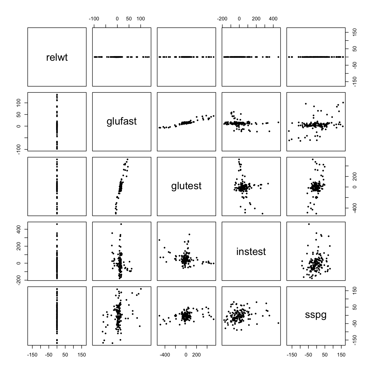
# within-group standard deviations
print(f1)
## relwt glufast glutest instest sspg
## 0.1195937 36.8753901 150.7536138 102.2913665 65.8125752# inverses of within-group standard deviations
scaling0 <- scaling
print(scaling0)## [,1] [,2] [,3] [,4] [,5]
## [1,] 8.361643 0.00000000 0.00000000 0.000000000 0.00000000
## [2,] 0.000000 0.02711836 0.00000000 0.000000000 0.00000000
## [3,] 0.000000 0.00000000 0.00663334 0.000000000 0.00000000
## [4,] 0.000000 0.00000000 0.00000000 0.009775996 0.00000000
## [5,] 0.000000 0.00000000 0.00000000 0.000000000 0.01519466The object scaling will be redefined twice as the function proceeds, each time by multiplication on the right, concluding with the member named scaling of the ‘lda’ object. We’ll denote these redefinitions \(S_1\) and \(S_2\) and store the three definitions as scaling0, scaling1, and scaling2 for unambiguous illustrations. These matrices act on the columns of \({X_0}\), which induces a two-sided action on \(C_W\): \(\frac{1}{n}({X_0}S)^\top({X_0}S)=S^\top C_WS\). The effect of \(S_0\) is to standardize the variables, so that the covariance matrix of the transformed data \({X_0}S_0\) is the within-group correlation matrix \(R_W\) of \({X_0}\). The effect is also evident from a comparison of the pairwise scatterplots:
# within-group correlation matrix
print(cor(x - group.means[g, ]))
## relwt glufast glutest instest sspg
## relwt 1.00000000 -0.09623213 -0.1607280 0.1070926 0.3926726
## glufast -0.09623213 1.00000000 0.9264021 -0.2513436 0.3692349
## glutest -0.16072796 0.92640213 1.0000000 -0.2494804 0.3633879
## instest 0.10709258 -0.25134359 -0.2494804 1.0000000 0.2145095
## sspg 0.39267262 0.36923495 0.3633879 0.2145095 1.0000000# within-group covariance matrix after standardization
print(cov((x - group.means[g, ]) %*% scaling))## [,1] [,2] [,3] [,4] [,5]
## [1,] 1.00000000 -0.09623213 -0.1607280 0.1070926 0.3926726
## [2,] -0.09623213 1.00000000 0.9264021 -0.2513436 0.3692349
## [3,] -0.16072796 0.92640213 1.0000000 -0.2494804 0.3633879
## [4,] 0.10709258 -0.25134359 -0.2494804 1.0000000 0.2145095
## [5,] 0.39267262 0.36923495 0.3633879 0.2145095 1.0000000# within-group centered data after standardization
pairs((x - group.means[g, ]) %*% scaling, asp = 1, pch = 19, cex = .5)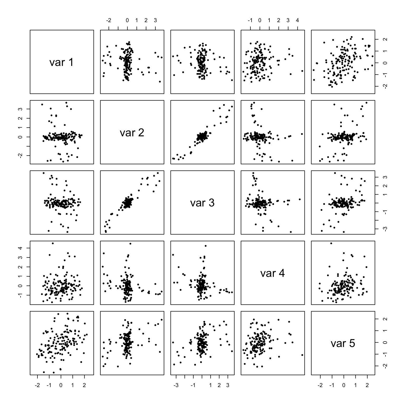
variable sphering and the Mahalanobis distance
The next step in the procedure is the signature transformation of LDA. Whereas \(S_0\) removes the scales of the variables, leaving them each with unit variance but preserving their correlations, the role of \(S_1\) is to additionally remove these correlations. Viewing the set of cases within each group as a cloud of \(n_k\) points in \(\mathbb{R}^p\), \(S_0\) stretches or compresses each cloud along its coordinate axes, while \(S_1\) will stretch or compress it along its principal components. The resulting aggregate point cloud will have within-group covariance \(I_n\) (the identity matrix), indicating unit variance and no correlation among its variables; according to these summary statistics, then, it is rotationally symmetric. Accordingly, the column action of \(S_1\) is called a sphering transformation, while the distances among the transformed points are called their Mahalanobis distances after their originator. See this SO answer by whuber for a helpful illustration of the transformation. Its importance is illustrated in Chapter 11 of Greenacre’s Biplots in Practice (p. 114).
\(S_1\) is calculated differently for different choices of method (see the documentation ?MASS::lda). For simplicity, the code chunk below follows the "mle" method.
As hinted in the previous paragraph, the process of obtaining a sphering transformation is closely related to principal components analysis. One can be calculated via eigendecomposition of the standardized within-group covariance matrix or, equivalently, via singular value decomposition of the standardized within-group centered data \(\hat{X}=X_0 S_0\).5 lda.default() performs SVD on \(\hat{X}\), scaled by \(\frac{1}{\sqrt{n}}\) so that the scatter matrix is \(R_W\):
fac <- 1/n # excise conditional case `method == "moment"`
X <- sqrt(fac) * (x - group.means[g,  ]) %*% scaling
X.s <- svd(X, nu = 0L)
rank <- sum(X.s$d > tol)
if(rank == 0L) stop("rank = 0: variables are numerically constant")
if(rank < p) warning("variables are collinear")
scaling <- scaling %*% X.s$v[, 1L:rank] %*% diag(1/X.s$d[1L:rank],,rank)
Taking the SVD to be \(\frac{1}{\sqrt{n}}\hat{X}=\hat{U}\hat{D}\hat{V}^\top\), the sphering matrix is \(S_1=S_0\hat{V}{\hat{D}}^{-1}\).
The alternative calculation is \(S_1=S_0\hat{V}{\hat{\Lambda}}^{-1/2}\), where \(\hat{C}=\hat{V}\hat{\Lambda}{\hat{V}}^\top\) is the eigendecomposition of the covariance matrix of \(\hat{X}\) so that \(\hat{V}\) is the same and \(\hat{\Lambda}={\hat{D}}^{1/2}\). (\({\hat{C}}^{-1/2}=\hat{V}{\hat{\Lambda}}^{-1/2}{\hat{V}}^\top\) is called the symmetric square root of \(\hat{C}\).)
Note that the signs of the columns are arbitrary, as in PCA. The difference in absolute values is due to stats::cov() treating \(\hat{X}\) as a sample rather than a population, dividing the scatter matrix \(\hat{X}^\top \hat{X}\) by \(\frac{1}{n-1}\) rather than by \(\frac{1}{n}\).
# standardized within-group centered data
Xhat <- (x - group.means[g,  ]) %*% scaling0
# eigendecomposition of covariance
E <- eigen(cov(Xhat))
# sphering matrix (alternative calculation)
scaling0 %*% E$vectors %*% diag(1/sqrt(E$values))
## [,1] [,2] [,3] [,4] [,5]
## [1,] -0.259027622 4.3010514864 5.4856218279 -6.620668927 -2.079154922
## [2,] 0.011804714 -0.0010406454 -0.0019199260 -0.013949375 0.070663381
## [3,] 0.002888749 -0.0004202234 -0.0008316344 -0.002406702 -0.017886747
## [4,] -0.001393182 0.0037523667 -0.0081405500 -0.005925590 -0.000197695
## [5,] 0.003470018 0.0076467225 -0.0008602899 0.018031665 0.001957544# sphering matrix
scaling1 <- scaling
print(scaling1)## [,1] [,2] [,3] [,4] [,5]
## [1,] 0.259925467 4.315959855 -5.5046361720 -6.643617588 2.0863617201
## [2,] -0.011845632 -0.001044253 0.0019265809 -0.013997727 -0.0709083156
## [3,] -0.002898762 -0.000421680 0.0008345171 -0.002415044 0.0179487460
## [4,] 0.001398012 0.003765373 0.0081687669 -0.005946129 0.0001983803
## [5,] -0.003482045 0.007673228 0.0008632718 0.018094166 -0.0019643291The sphered within-group centered data now have identity within-group covariance matrix, up to a reasonable tolerance. The sphered coordinates are true to their name, as along each pair of variable coordinates the point cloud exhibits no elliptical tendencies.
While rank is 5 (\(=p\)) at this stage, indicating that variation is detected in each of the variables, the final computational step will determine the rank of the LDA itself in terms of the transformed group centroids.
# within-group covariance matrix after sphering
print(cov((x - group.means[g, ]) %*% scaling))
## [,1] [,2] [,3] [,4] [,5]
## [1,] 1.006944e+00 3.762724e-16 -5.781689e-16 5.015188e-16 1.113855e-15
## [2,] 3.762724e-16 1.006944e+00 1.892763e-15 4.976970e-16 5.560143e-16
## [3,] -5.781689e-16 1.892763e-15 1.006944e+00 -9.853124e-16 -1.180559e-15
## [4,] 5.015188e-16 4.976970e-16 -9.853124e-16 1.006944e+00 1.095132e-15
## [5,] 1.113855e-15 5.560143e-16 -1.180559e-15 1.095132e-15 1.006944e+00# within-group centered data after sphering
pairs((x - group.means[g, ]) %*% scaling, asp = 1, pch = 19, cex = .5)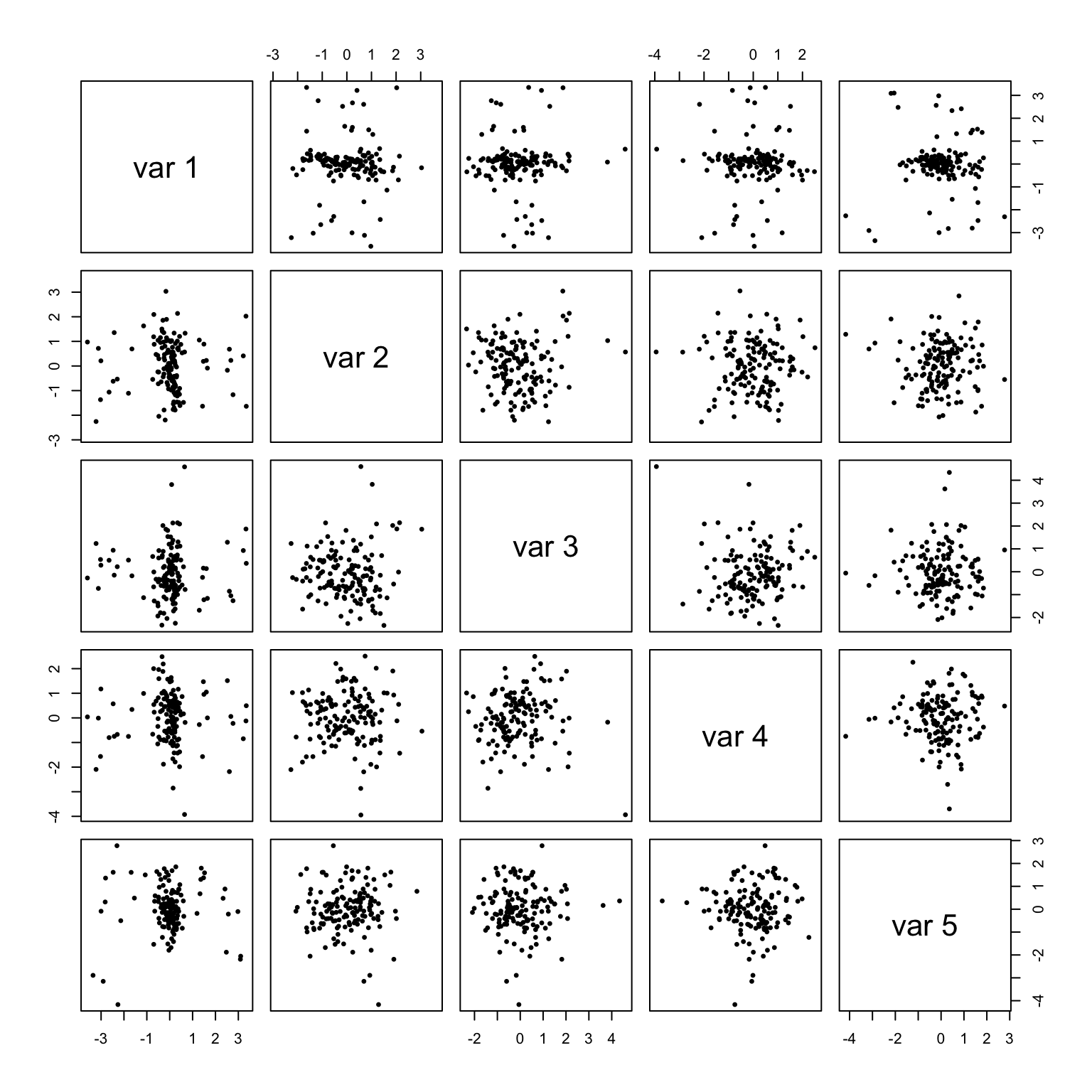
# number of variables that contribute to the sphered data
print(rank)
## [1] 5sphering-transformed group centroids and discriminant coefficients
The original problem of LDA was to eigendecompose \({C_W}^{-1}C_B\), where \(C_B=\frac{1}{q}Y^\top Y\) is the between-groups covariance matrix derived from the centered group centroids \(Y=G\overline{X}-\mathbb{1}_{n\times 1}\overline{x}\in\mathbb{R}^{n\times p}\) using the data centroid \(\overline{x}=\frac{1}{n}\mathbb{1}_{1\times n}X\in\mathbb{R}^{1\times p}\) (and duplicated according to the group counts).
lda.default() relies on an equivalent calculation \(C_B=\frac{1}{q}\overline{Y}^\top\overline{Y}\), using \(\overline{Y}=N(\overline{X}-\mathbb{1}_{q\times 1}\overline{x})\), which explicitly weights the centered group centroids by the group counts and produces the same scatter matrix as \(Y\).
Under the transformed coordinates \({X_0}S_1\), the matrix quotient to be eigendecomposed becomes \[\textstyle({S_1}^\top C_WS_1)^{-1}({S_1}^\top C_BS_1)=I_p{S_1}^\top C_BS_1=\frac{1}{q}(YS_1)^\top(YS_1)=\frac{1}{q}(\overline{Y}S_1)^\top(\overline{Y}S_1),\]
the between-groups covariance calculated from the sphering-transformed centered group centroids.6
This is the first calculation using \(C_B\), which is how lda.default() can wait until here to calculate the data centroid xbar.
xbar <- colSums(proportions %*% group.means) # sub `proportions` for `prior`
fac <- 1/(ng - 1) # excise conditional case `method == "mle"`
X <- sqrt((n * proportions)*fac) * # sub `proportions` for `prior`
  scale(group.means, center = xbar, scale = FALSE) %*% scaling
X.s <- svd(X, nu = 0L)
rank <- sum(X.s$d > tol * X.s$d[1L])
if(rank == 0L) stop("group means are numerically identical")
scaling <- scaling %*% X.s$v[, 1L:rank]
# excise conditional case `is.null(dimnames(x))`
dimnames(scaling) <- list(colnames(x), paste("LD", 1L:rank, sep = ""))
dimnames(group.means)[[2L]] <- colnames(x)
The rank now indicates the number of dimensions in the SVD of the sphering-transformed group centroids, which can be no more than \(q-1\).
The final reassignment of scaling gives \(S_2\), the raw discriminant coefficients that express the discriminant coordinates of the centroids (and of the original data) as linear combinations of the centered variable coordinates. In practice, these discriminant coordinates are returned by the predict() method for ‘lda’ objects, MASS:::predict.lda(), and this is demonstrated to conclude the post:
# number of dimensions in the sphering-transformed group centroid SVD
print(rank)
## [1] 2# discriminant coefficients
scaling2 <- scaling
print(scaling2)## LD1 LD2
## relwt 1.3767523932 -3.823906854
## glufast -0.0340023755 0.037018266
## glutest 0.0127085491 -0.007166541
## instest -0.0001032987 -0.006238295
## sspg 0.0042877747 0.001145987# discriminant coordinates of centered group centroids
print((group.means - matrix(1, ng, 1) %*% t(xbar)) %*% scaling2)## LD1 LD2
## Normal -1.7683547 0.4043199
## Chemical_Diabetic 0.3437412 -1.3910995
## Overt_Diabetic 3.6975842 0.5864022# as recovered using `predict.lda()`
fit <- MASS::lda(group ~ ., heplots::Diabetes)
print(predict(fit, as.data.frame(fit$means))$x)## LD1 LD2
## Normal -1.7499658 0.4001154
## Chemical_Diabetic 0.3401666 -1.3766336
## Overt_Diabetic 3.6591334 0.5803043(The slight discrepancy between the manually calculated coordinates and those returned by predict() is left as an exercise for the reader.)
If you use ordination and ggplot2, not necessarily together (yet), i’d be grateful for your feedback, too!↩
My exposition here assumes the covariances were calculated from a population rather than a sample perspective, but this introduces discrepancies in a few places.↩
To see the source code for an object included in but not exported by a package, use three colons instead of two, e.g.
MASS:::lda.default.↩I’ve been searching for a history of the 1970s change from categorizing diabetes as “clinical” versus “overt” to the present-day categories of “type 1” and “type 2”. Recommended reading is very welcome.↩
These are equivalent because the matrix factors \(U\) and \(V\) of an SVD of any matrix \(Z\) are the eigenvector matrices of \(ZZ^\top\) and of \(Z^\top Z\), respectively.↩
These are not “sphered” centered group centroids because the sphering transformation is specific to the within-group centered data.↩