how to calculate aesthetics in a ggplot2 extension

how to use computed variables

One of the many subtle features of ggplot2 is the ability to pass variables to aesthetics that are not present in the data but rather are computed internally by a statistical transformation (stat). For users, the documentation for this feature illustrates the use of stat(<variable>) (previously ..<variable>.., since upgraded to after_stat(<variable>)) in an aesthetic specification.

Some stats do this by default. For example, the count stat sends its computed count to both coordinate aesthetics by default. Because it requires exactly one of them to be specified, only the other receives the count:

print(StatCount$default_aes)

## Aesthetic mapping: 
## * `x`      -> `after_stat(count)`
## * `y`      -> `after_stat(count)`
## * `weight` -> 1

print(StatCount$required_aes)

## [1] "x|y"

This is how the count stat supports its companion graphical element, the bar geom. This geom needs both the categorical variable from the data and the count variable computed by the stat in order to produce a (frequency) bar plot. The code below, which tallies the cars in the mpg data set by classification, makes some of this implicit control explicit:

table(mpg$class)

## 
##    2seater    compact    midsize    minivan     pickup subcompact        suv 
##          5         47         41         11         33         35         62

ggplot(mpg) +
  stat_count(aes(x = class, y = after_stat(count)))

More than calling single variables, after_stat() can also perform and return calculations involving these variables. For example, to produce a relative (frequency) bar plot of the classified cars, the y variable needs not the raw counts but what proportion they make up of the total Note the y axis range in this revised plot:

ggplot(mpg) +
  stat_count(aes(x = class, y = after_stat(count / sum(count)))) +
  scale_y_continuous(labels = scales::percent)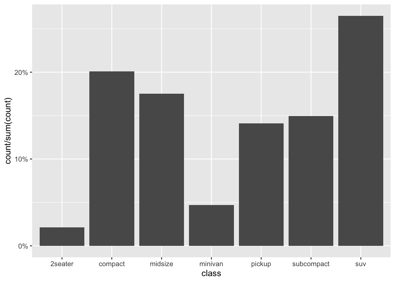

More illustrations can be found in the aforelinked documentation, which are reasonably intuitive from a user’s perspective. Though it’s not immediately evident where after_stat() locates these computed variables and what the limits are to its ability to perform calculations on them. The documentation help(after_stat) thoroughly tracks the processing of an aesthetic from start to stat to scale, but again with users in mind.

how to make computed variables

Another exceptional feature of ggplot2 is its extensibility. Users with specialized plotting needs can, with limited exposure to the package internals, write stats and geoms that produce new types of plots. Because they are extensions, rather than standalone packages, they benefit from the grammatical rigor of ggplot2 and often combine well with existing stats and geoms.

From a developer’s perspective, especially someoene like myself with limited low-level programming experience, computed variables can appear mysterious. Yet, they are perhaps the single easiest feature to include in a ggplot2 extension.

To illustrate, consider this simplified custom stat from the vignette on extending ggplot2:

# a custom ggproto stat to fit a linear model to data
StatLm <- ggproto("StatLm", Stat, 
  required_aes = c("x", "y"),
  
  compute_group = function(data, scales, params, n = 100, formula = y ~ x) {
    rng <- range(data$x, na.rm = TRUE)
    grid <- data.frame(x = seq(rng[1], rng[2], length = n))
    
    mod <- lm(formula, data = data)
    grid$y <- predict(mod, newdata = grid)
    
    grid
  }
)
# a corresponding stat layer
stat_lm <- function(mapping = NULL, data = NULL, geom = "line",
                    position = "identity", na.rm = FALSE, show.legend = NA, 
                    inherit.aes = TRUE, n = 50, formula = y ~ x, 
                    ...) {
  layer(
    stat = StatLm, data = data, mapping = mapping, geom = geom, 
    position = position, show.legend = show.legend, inherit.aes = inherit.aes,
    params = list(n = n, formula = formula, na.rm = na.rm, ...)
  )
}
# an illustration of the stat
ggplot(mpg, aes(displ, hwy)) + 
  geom_point() + 
  stat_lm()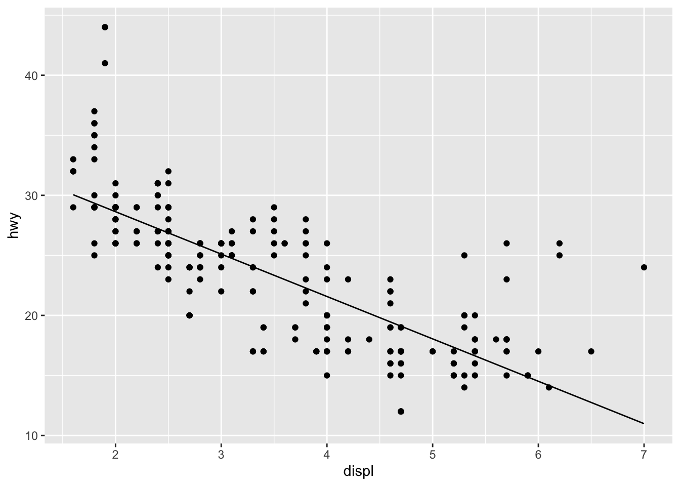

The computation step of this linear model stat returns a data frame grid with two columns: a regular sequence of x values spanning the range of engine displacement volumes in the data set, whose number are determined by the parameter n; and the predicted highway speed y at each, according to the internally-fitted model mod. Notice that the data returned by the stat is differently sized than the data passed to it:

dim(mpg)

## [1] 234  11

head(mpg)

## # A tibble: 6 x 11
##   manufacturer model displ  year   cyl trans      drv     cty   hwy fl    class 
##   <chr>        <chr> <dbl> <int> <int> <chr>      <chr> <int> <int> <chr> <chr> 
## 1 audi         a4      1.8  1999     4 auto(l5)   f        18    29 p     compa…
## 2 audi         a4      1.8  1999     4 manual(m5) f        21    29 p     compa…
## 3 audi         a4      2    2008     4 manual(m6) f        20    31 p     compa…
## 4 audi         a4      2    2008     4 auto(av)   f        21    30 p     compa…
## 5 audi         a4      2.8  1999     6 auto(l5)   f        16    26 p     compa…
## 6 audi         a4      2.8  1999     6 manual(m5) f        18    26 p     compa…

data <- transform(mpg, x = displ, y = hwy)[, c("x", "y")]
dim(StatLm$compute_group(data))

## [1] 100   2

head(StatLm$compute_group(data))

##          x        y
## 1 1.600000 30.04871
## 2 1.654545 29.85613
## 3 1.709091 29.66355
## 4 1.763636 29.47098
## 5 1.818182 29.27840
## 6 1.872727 29.08582

The predictions computed by the stat are estimates of conditional means (under a set of assumptions outside the scope of this example), and it’s often useful for a plot to encode the uncertainty of those estimates graphically. First, the uncertainty must be computed by the stat, as below by including a standard error calculation at the predict() step:

# the linear model ggproto stat, with a computed variable for standard error
StatLm <- ggproto("StatLm", Stat, 
  required_aes = c("x", "y"),
  
  compute_group = function(data, scales, params, n = 100, formula = y ~ x) {
    rng <- range(data$x, na.rm = TRUE)
    grid <- data.frame(x = seq(rng[1], rng[2], length = n))
    
    mod <- lm(formula, data = data)
    pred <- predict(mod, newdata = grid, se.fit = TRUE)
    grid$y <- pred$fit
    grid$yse <- pred$se.fit
    
    grid
  }
)

In addition to x and y, the data frame computed by the stat now includes a yse column, containing the standard errors of the predicted means contained in y:

head(StatLm$compute_group(data))

##          x        y       yse
## 1 1.600000 30.04871 0.4420916
## 2 1.654545 29.85613 0.4333956
## 3 1.709091 29.66355 0.4247865
## 4 1.763636 29.47098 0.4162698
## 5 1.818182 29.27840 0.4078513
## 6 1.872727 29.08582 0.3995371

Paired with the ribbon geom, this stat can now produce a 95% confidence band for the mean highway speeds predicted for the full range of engine displacement volumes¹:

ggplot(mpg, aes(displ, hwy)) + 
  geom_point() + 
  stat_lm(geom = "ribbon", alpha = .2,
          aes(ymin = after_stat(y - 2 * yse), ymax = after_stat(y + 2 * yse))) +
  stat_lm()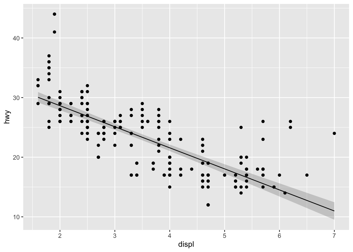

As a concluding caveat, i haven’t dug far enough into the ggplot2 source code to know exactly how the expressions fed to after_stat() are evaluated. In principle, if a stat returns the data frame ret, then after_stat(<expression>) is evaluated like with(ret, <expression>). In particular, objects in the global environment are recognized:

z <- 3
ggplot(mpg, aes(displ, hwy)) + 
  geom_point() + 
  stat_lm(geom = "ribbon", alpha = .2,
          aes(ymin = after_stat(y - z * yse), ymax = after_stat(y + z * yse))) +
  stat_lm()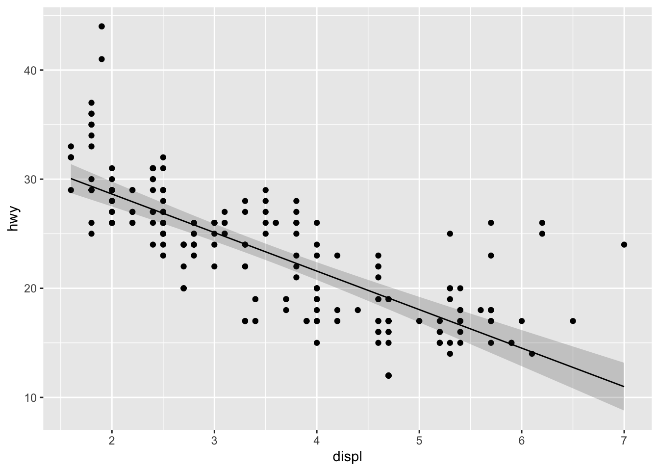

Finally, to document new computed variables, the natural thing to do is mimic the documentation of those in the main package—for example, help(stat_count). Here is some minimal documentation for the standard error variable:

#' @section Computed variables:
#' \describe{
#'   \item{yse}{standard error of predicted means}
#' }

In a pinch, the computed variables may be gleaned from the source code for the relevant compute method of the stat—if the internals are concise and tidy enough. Since the count stat performs group-wise tallies, the method to inspect is StatCount$compute_group():

print(StatCount$compute_group)

## <ggproto method>
##   <Wrapper function>
##     function (...) 
## f(..., self = self)
## 
##   <Inner function (f)>
##     function (self, data, scales, width = NULL, flipped_aes = FALSE) 
## {
##     data <- flip_data(data, flipped_aes)
##     x <- data$x
##     weight <- data$weight %||% rep(1, length(x))
##     width <- width %||% (resolution(x) * 0.9)
##     count <- as.numeric(tapply(weight, x, sum, na.rm = TRUE))
##     count[is.na(count)] <- 0
##     bars <- new_data_frame(list(count = count, prop = count/sum(abs(count)), 
##         x = sort(unique(x)), width = width, flipped_aes = flipped_aes), 
##         n = length(count))
##     flip_data(bars, flipped_aes)
## }

Indeed, count is not the only variable computed by the stat. The code is specialized, but it’s clear that some additional variables—prop, x, and width—are computed as well. The last two are meant for the paired geom; they could be invoked using after_stat(), but this is not their intended role, and they are not documented among the computed stats. The documentation serves dual purposes: enable intended use, and avert unintended use.

conclusion

To sum up the topic for ggplot2 extension developers:

• A computed variable is just a column of the data frame returned by Stat*$compute_*().
• Any expression involving such computed variables can be passed as a calculated aesthetic via aes(<aes> = after_stat(<expr>)).
• Users should be able to learn about computed variables in a specific Computed variables section of the documentation for such a stat.