Restrict planar data to the boundary points of its convex hull, or of nested convex hulls containing specified fractions of points.
Usage
stat_chull(
  mapping = NULL,
  data = NULL,
  geom = "polygon",
  position = "identity",
  show.legend = NA,
  inherit.aes = TRUE,
  ...
)

stat_peel(
  mapping = NULL,
  data = NULL,
  geom = "polygon",
  position = "identity",
  num = NULL,
  by = 1L,
  breaks = c(0.5),
  cut = c("above", "below"),
  show.legend = NA,
  inherit.aes = TRUE,
  ...
)
Arguments
- mapping
Set of aesthetic mappings created by
aes(). If specified andinherit.aes = TRUE(the default), it is combined with the default mapping at the top level of the plot. You must supplymappingif there is no plot mapping.- data
The data to be displayed in this layer. There are three options:
If
NULL, the default, the data is inherited from the plot data as specified in the call toggplot().A
data.frame, or other object, will override the plot data. All objects will be fortified to produce a data frame. Seefortify()for which variables will be created.A
functionwill be called with a single argument, the plot data. The return value must be adata.frame, and will be used as the layer data. Afunctioncan be created from aformula(e.g.~ head(.x, 10)).- geom
The geometric object to use to display the data for this layer. When using a
stat_*()function to construct a layer, thegeomargument can be used to override the default coupling between stats and geoms. Thegeomargument accepts the following:A
Geomggproto subclass, for exampleGeomPoint.A string naming the geom. To give the geom as a string, strip the function name of the
geom_prefix. For example, to usegeom_point(), give the geom as"point".For more information and other ways to specify the geom, see the layer geom documentation.
- position
A position adjustment to use on the data for this layer. This can be used in various ways, including to prevent overplotting and improving the display. The
positionargument accepts the following:The result of calling a position function, such as
position_jitter(). This method allows for passing extra arguments to the position.A string naming the position adjustment. To give the position as a string, strip the function name of the
position_prefix. For example, to useposition_jitter(), give the position as"jitter".For more information and other ways to specify the position, see the layer position documentation.
- show.legend
logical. Should this layer be included in the legends?
NA, the default, includes if any aesthetics are mapped.FALSEnever includes, andTRUEalways includes. It can also be a named logical vector to finely select the aesthetics to display. To include legend keys for all levels, even when no data exists, useTRUE. IfNA, all levels are shown in legend, but unobserved levels are omitted.- inherit.aes
If
FALSE, overrides the default aesthetics, rather than combining with them. This is most useful for helper functions that define both data and aesthetics and shouldn't inherit behaviour from the default plot specification, e.g.annotation_borders().- ...
Additional arguments passed to
ggplot2::layer().- num
A positive integer; the number of hulls to peel. Pass
Inffor all hulls.- by
A positive integer; with what frequency to include consecutive hulls, pairs with
num.- breaks
A numeric vector of fractions (between
0and1) of the data to contain in each hull; overridden bynum.- cut
Character; one of
"above"and"below", indicating whether each hull should contain at least or at mostbreaksof the data, respectively.
Details
As used in a ggplot2 vignette,
stat_chull() restricts a dataset with x and y variables to the points
that lie on its convex hull.
Building on this, stat_peel() returns hulls from a convex hull peeling:
a subset of sequentially removed hulls containing specified fractions of
the data.
Multidimensional position aesthetics
This statistical transformation is compatible with the convenience function
aes_coord().
Some transformations (e.g. stat_center()) commute with projection to the
lower (1 or 2)-dimensional biplot space. If they detect aesthetics of the
form ..coord[0-9]+, then ..coord1 and ..coord2 are converted to x and
y while any remaining are ignored.
Other transformations (e.g. stat_spantree()) yield different results in a
lower-dimensional biplot when they are computed before versus after
projection. If the stat layer detects these aesthetics, then the
transformation is performed before projection, and the results in the first
two dimensions are returned as x and y.
A small number of transformations (stat_rule()) are incompatible with
these aesthetics but will accept aes_coord() without warning.
Computed variables
These are calculated during the statistical transformation and can be accessed with delayed evaluation.
hullthe position of
breaksthat defines each hullfracthe value of
breaksthat defines each hullpropthe actual proportion of data within each hull
References
Barnett V (1976) "The Ordering of Multivariate Data". Journal of the Royal Statistical Society: Series A (General), 139(3): 318–344. doi:10.2307/2344839
See also
Other stat layers:
stat_bagplot(),
stat_center(),
stat_cone(),
stat_depth(),
stat_rule(),
stat_scale(),
stat_spantree()
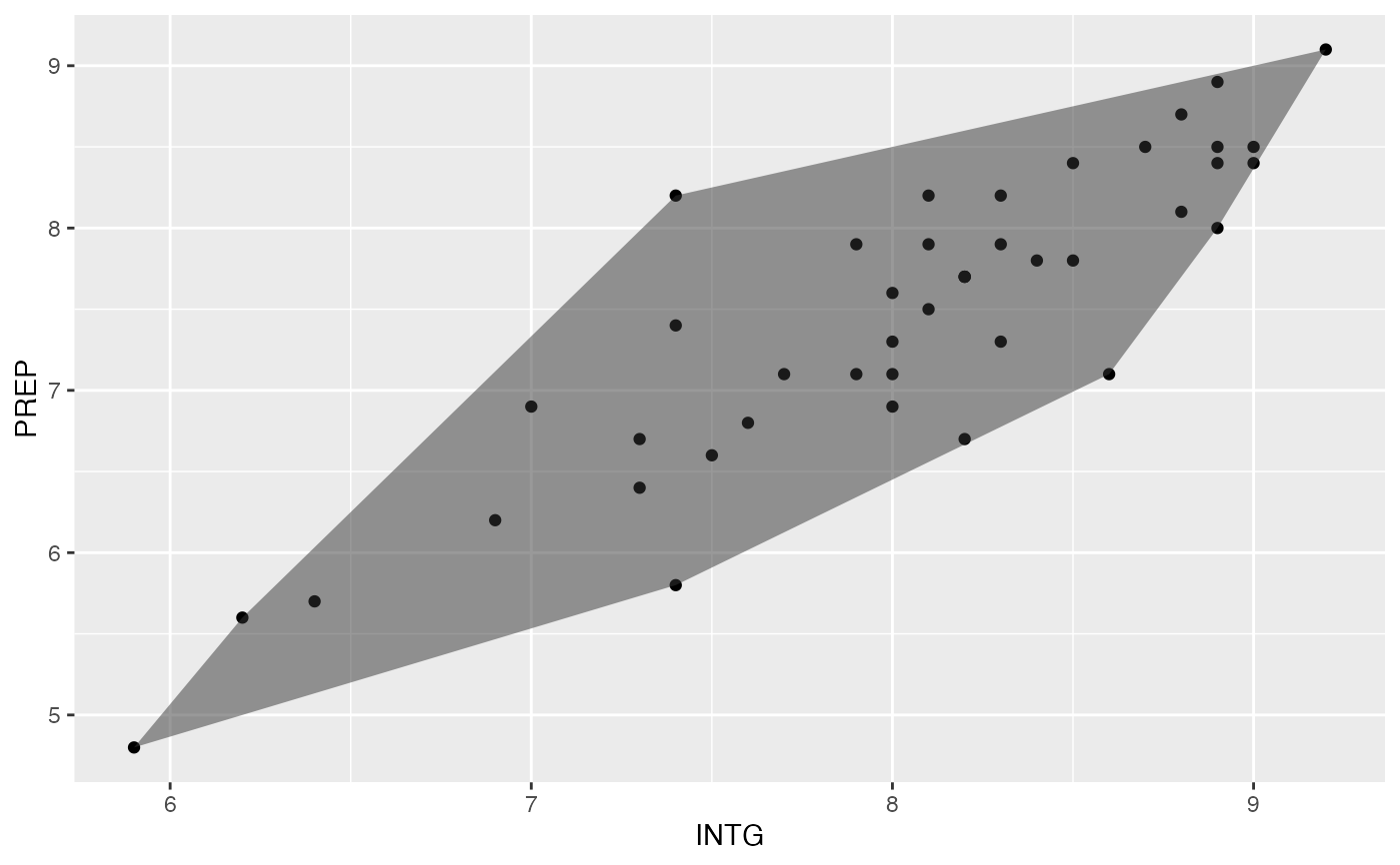
Examples
ggplot(USJudgeRatings, aes(x = INTG, y = PREP)) +
geom_point() +
stat_chull(alpha = .5)
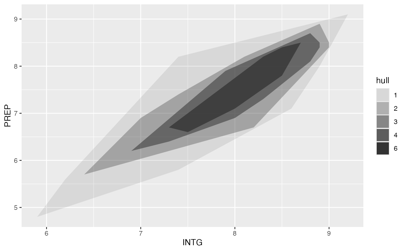
 ggplot(USJudgeRatings, aes(x = INTG, y = PREP)) +
stat_peel(
aes(alpha = after_stat(hull)),
breaks = seq(.1, .9, .2)
)
#> Warning: Using alpha for a discrete variable is not advised.
ggplot(USJudgeRatings, aes(x = INTG, y = PREP)) +
stat_peel(
aes(alpha = after_stat(hull)),
breaks = seq(.1, .9, .2)
)
#> Warning: Using alpha for a discrete variable is not advised.
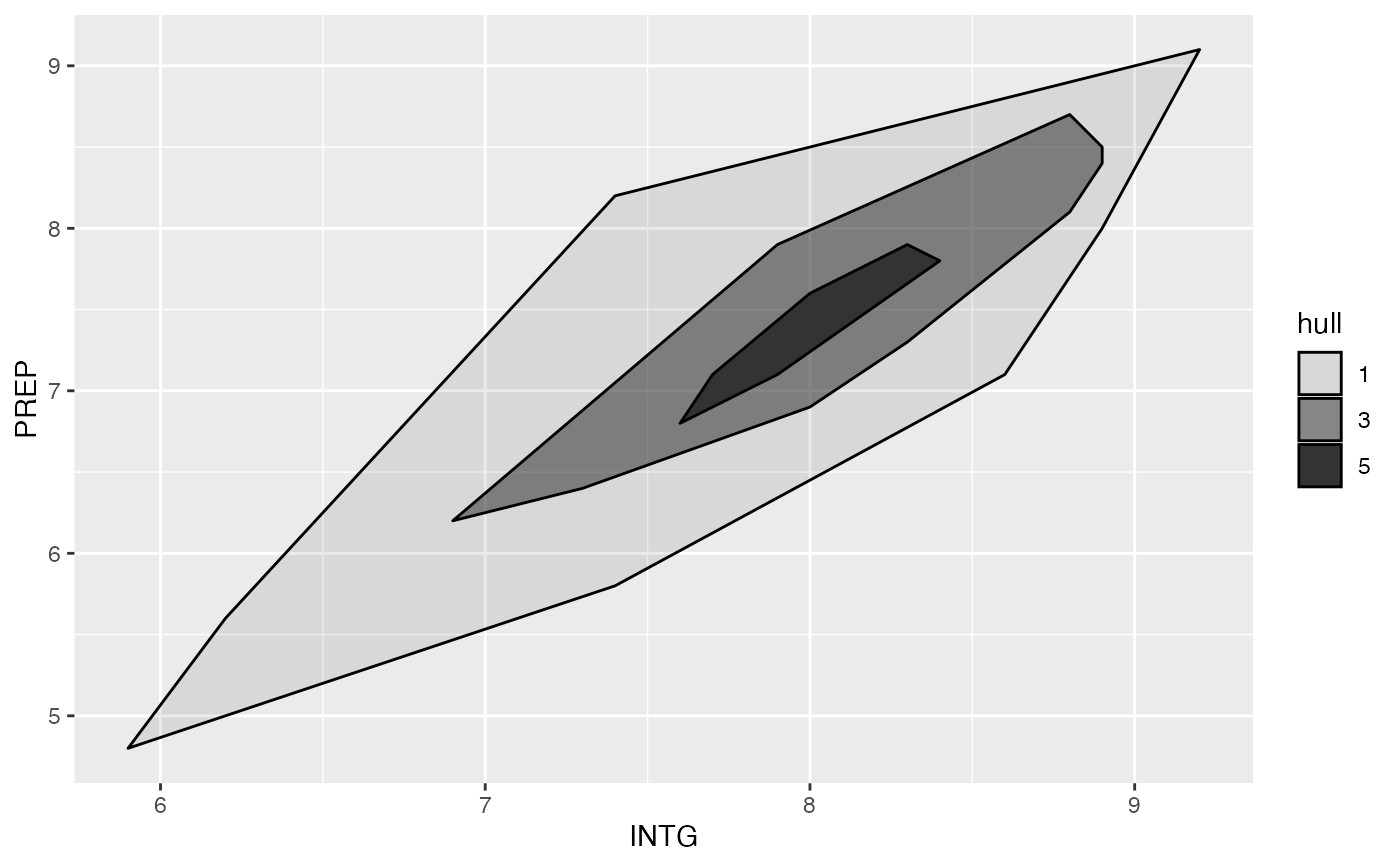
 ggplot(USJudgeRatings, aes(x = INTG, y = PREP)) +
stat_peel(
aes(alpha = after_stat(hull)),
num = 6, by = 2, color = "black"
)
#> Warning: Using alpha for a discrete variable is not advised.
ggplot(USJudgeRatings, aes(x = INTG, y = PREP)) +
stat_peel(
aes(alpha = after_stat(hull)),
num = 6, by = 2, color = "black"
)
#> Warning: Using alpha for a discrete variable is not advised.
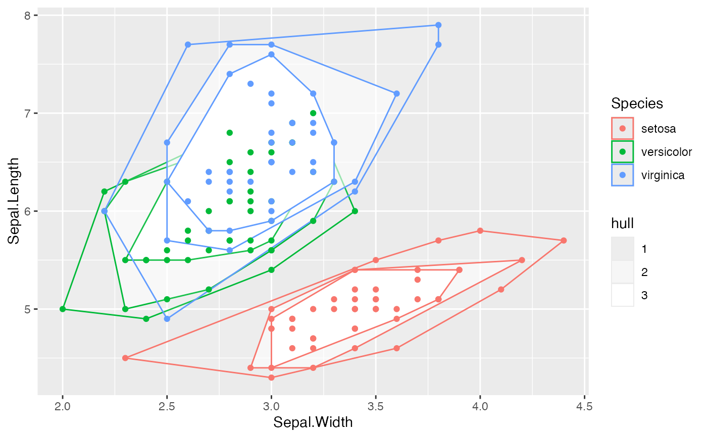
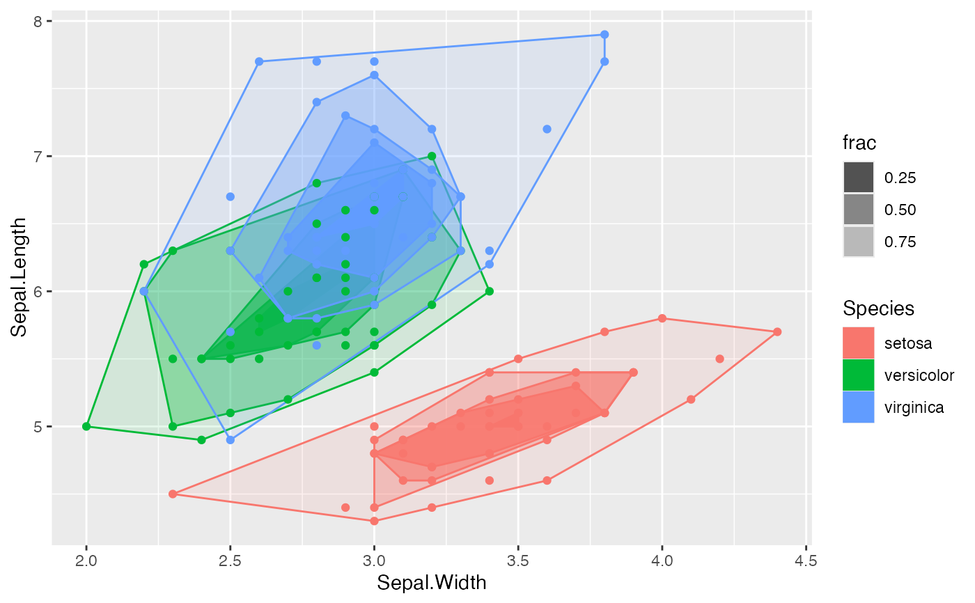
 # specify fractions of points
ggplot(iris, aes(Sepal.Width, Sepal.Length, color = Species)) +
stat_peel(aes(fill = Species, alpha = after_stat(frac)),
breaks = seq(.1, .9, .2)) +
scale_alpha_continuous(trans = scales::reverse_trans()) +
geom_point()
# specify fractions of points
ggplot(iris, aes(Sepal.Width, Sepal.Length, color = Species)) +
stat_peel(aes(fill = Species, alpha = after_stat(frac)),
breaks = seq(.1, .9, .2)) +
scale_alpha_continuous(trans = scales::reverse_trans()) +
geom_point()
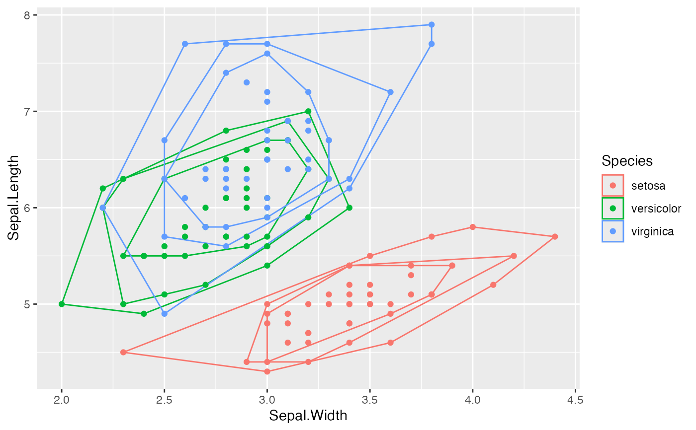
 # specify number of peels
ggplot(iris, aes(Sepal.Width, Sepal.Length, color = Species)) +
stat_peel(fill = "transparent", num = 3) +
geom_point()
# specify number of peels
ggplot(iris, aes(Sepal.Width, Sepal.Length, color = Species)) +
stat_peel(fill = "transparent", num = 3) +
geom_point()
 # mapping to opacity overrides transparency
ggplot(iris, aes(Sepal.Width, Sepal.Length, color = Species)) +
stat_peel(aes(alpha = after_stat(hull)), fill = "transparent", num = 3) +
geom_point()
#> Warning: Using alpha for a discrete variable is not advised.
# mapping to opacity overrides transparency
ggplot(iris, aes(Sepal.Width, Sepal.Length, color = Species)) +
stat_peel(aes(alpha = after_stat(hull)), fill = "transparent", num = 3) +
geom_point()
#> Warning: Using alpha for a discrete variable is not advised.