the mapper construction in base R

precap

Briefly, here is some notation for the elements of the construction, adapted from Mémoli and Singhal:

• \(X\) – the point cloud (a finite metric space)
• \(f:X\to Z\) – the lens function from \(X\) to the lens space \(Z\)
• \(\mathcal{U}=\{U_i\}\) – the cover of \(f(X)\), usually inferred from (and used interchangeably with) a finite cover of a subset \(S\subset Z\) that contains \(f(X)\)
• \(\delta:X\times X\to\mathbb{R}_{\geq0}\) – the distance metric on \(X\)
• \(C:\mathcal{M}\to\mathcal{P}\) – the clustering method, based on \(\delta\), that sends metric spaces \(Y\subseteq X\) to partitions of their elements
• \(\mathcal{V}=\{V_{ij}\}=\bigcup_i{C(f^{-1}(U_i))}\) – the refinement of the pullback cover \(\{f^{-1}\mathcal{U}\}\) of \(X\) obtained by partitioning each subset \(f^{-1}(U_i)\subset X\)
• \(N\) – the nerve of \(\mathcal{V}\), comprising a simplex for every non-empty intersection of sets in \(\mathcal{V}\)

construction

I’ll begin with probably the most common toy example, the noisy circle. Since this isn’t part of the construction per se, i’m allowing myself the vanity of invoking a manifold sampling package under development with two high school interns:

set.seed(2)
# point cloud
x <- tdaunif::sample_circle(n = 120, sd = .1)
x[, 2] <- x[, 2] + 1.5
print(head(x))

##                x         y
## [1,]  0.21900250 2.3144202
## [2,] -0.09167245 0.4182471
## [3,] -0.96604574 1.0946227
## [4,]  0.50825992 2.2572006
## [5,]  0.98900895 1.2088241
## [6,]  0.85559229 1.2699230

I’ve shifted the coordinates upward for downstream plotting purposes. Note that this point cloud \(X\) exists in \(\mathbb{R}^2\) but that i have not yet declared a distance metric \(\delta\) on \(X\).

The lens (or filter) \(f\) is usually (a) obtained via dimensionality reduction on the \(X\) or (b) taken to be a meaningful stratification variable of or function on \(X\). This example takes approach (a), projecting \(X\) to its first coordinate:

# lensed point cloud
f <- x[, 1]
print(head(f))

## [1]  0.21900250 -0.09167245 -0.96604574  0.50825992  0.98900895  0.85559229

For ease of visualization as well as personal preference, i’ll use a fixed-width interval cover \(\mathcal{U}=\{U_i\}\) with diameter half that of \(f(X)\) and 50% overlap, which comprises five sets. I like this sort of cover because it is (uniformly) 2-fold—every point of \(f(X)\) is contained in exactly two \(U_i\):

# cover interval length
d <- diff(range(f))*1/2
# cover interval centers
c <- seq(min(f), max(f), d/2)
# cover intervals
u <- cbind(x0 = c - d/2, x1 = c + d/2)
print(u)

##                x0           x1
## [1,] -1.748626379 -0.586016272
## [2,] -1.167321326 -0.004711219
## [3,] -0.586016272  0.576593835
## [4,] -0.004711219  1.157898888
## [5,]  0.576593835  1.739203942

The pullback cover \(f^{-1}(\mathcal{U})\) of \(X\) is a straightforward step that involves no choice on the users part, though note the use of <= and < to ensure (up to mechanical precision) that cover set boundaries are handled correctly:

# pullback cover sets
p <- apply(u, 1, function(u_i) which(u_i[1] <= f & f < u_i[2]))
names(p) <- paste0(seq(p), ":")
print(lapply(p, head))

## $`1:`
## [1]  3  9 10 11 15 19
## 
## $`2:`
## [1]  2  3  9 10 11 15
## 
## $`3:`
## [1]  1  2  4  7  8 12
## 
## $`4:`
## [1] 1 4 5 6 7 8
## 
## $`5:`
## [1]  5  6 17 20 29 30

To partition the preimages \(f^{-1}(U_i)\in f^{-1}(\mathcal{U})\), i’ve used the theoretically exceptional method of single-linkage hierarchical clustering, but with a dangerously naïve fixed cutoff at height \(\frac{1}{3}\):

# clustered pullback cover sets
cl <- function(p_i) {
  m <- cutree(hclust(dist(x[p_i, , drop = FALSE]), method = "single"), h = 1/3)
  lapply(unique(m), function(v_ij) p_i[which(m == v_ij)])
}
v <- unlist(lapply(p, cl), recursive = FALSE)
print(lapply(v, head))

## $`1:`
## [1]  3  9 10 11 15 19
## 
## $`2:`
## [1]  2  3  9 10 11 15
## 
## $`3:1`
## [1]  1  4  7 12 14 18
## 
## $`3:2`
## [1]  2  8 13 16 21 23
## 
## $`4:`
## [1] 1 4 5 6 7 8
## 
## $`5:`
## [1]  5  6 17 20 29 30

While the clusters \(V_{ij}\) will be encoded as vertices, higher-dimensional simplices will represent overlaps \(V_{ij}\cap V_{i'j'}\) among them (\(i\neq i'\)). Happily, because the cover is 2-fold, any lensed point \(f(x)\) lies in the intersection \(U_i\cap U_{i'}\) of at most two cover sets, so in this case we only have to worry about edges between pairs of vertices. Moreover, the only intersections to check are those between cover sets of adjacent indices \(i'\in\{i-1,i+1\}\):

# matrix of pairwise overlaps
b <- matrix(NA, nrow = 0, ncol = 2)
for (ij in seq(length(v) - 1)) {
  i <- as.integer(gsub(":.*$", "", names(v)[[ij]]))
  i1js <- grep(paste0("^", i + 1, ":"), names(v))
  for (i1j in i1js) {
    if (length(intersect(v[[ij]], v[[i1j]])) > 0) {
      b <- rbind(b, c(ij, i1j))
    }
  }
}
print(b)

##      [,1] [,2]
## [1,]    1    2
## [2,]    2    3
## [3,]    2    4
## [4,]    3    5
## [5,]    4    5
## [6,]    5    6

(It’s possible, just cumbersome, to handle arbitrary covers and arbitrarily high-dimensional simplices.)

visualization

The whole process is visualized below, also in base R (with the exception of a ColorBrewer palette), with comments separating the steps. To construct constituent frames of a gif or slideshow, just execute progressively more commented chunks from start to end.³

plot.new()
plot.window(c(-1.25, 1.25), c(-.25, 2.75), asp = 1)
# point cloud
points(x, pch = 19, cex = .5)
# lens
lines(x = c(-2, 2), y = c(0, 0), lty = 1)
rug(f, pos = 0)
# cover
u_cols <- RColorBrewer::brewer.pal(nrow(u), "Set1")
segments(
  x0 = u[, 1] + .015, x1 = u[, 2] - .015,
  y0 = c(-.1, -.2), col = u_cols, lwd = 3
)
l_nudge <- rep_len(c(T, F), length.out = nrow(u))
# pullback cover
rect(
  xleft = u[, 1] + .015, xright = u[, 2] - .015,
  ybottom = .15 + .2*l_nudge, ytop = 2.65 + .2*l_nudge,
  col = paste0(u_cols, "77"), border = NA
)
# nerve
n_lay <- t(sapply(seq_along(v), function(i) {
  apply(x[v[[i]], , drop = FALSE], 2, mean)
}))
for (i in seq(nrow(b))) lines(x = n_lay[b[i, ], 1], y = n_lay[b[i, ], 2])
points(x = n_lay[, 1], y = n_lay[, 2],
       pch = 21, cex = 2, lwd = 2, bg = "white",
       col = u_cols[as.integer(gsub("^([0-9]+)\\:.*$", "\\1", names(v)))])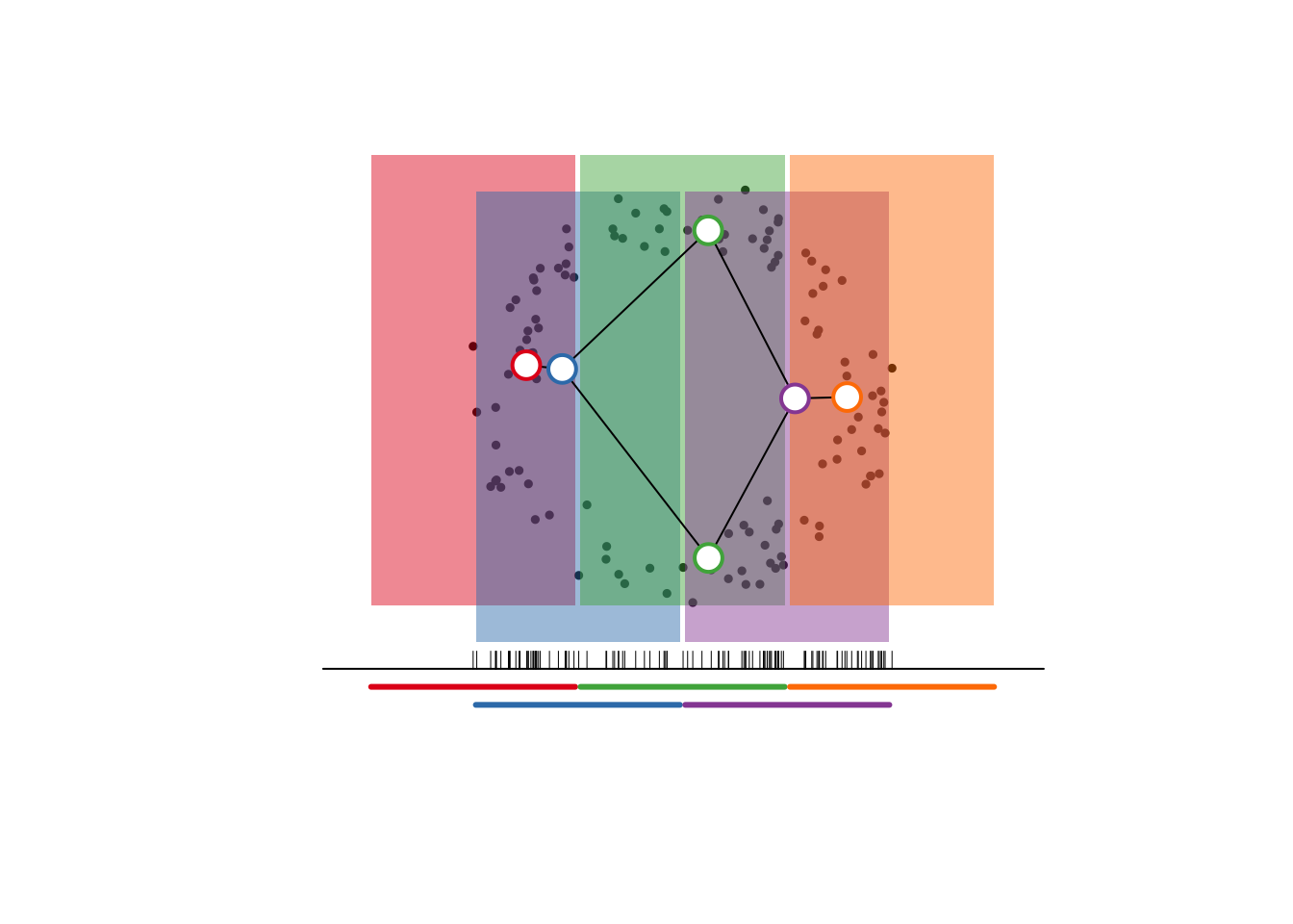

I’m pretty sure that this is the only visualization of mapper i’ve seen that

• comes from an implementation on a non-trivial point cloud and
• represents every step in the construction.

I general, it would be difficult to visualize the mapper internals like this, for example when \(Z\) isn’t low-enough-dimensional or \(f\) is not a linear projection of \(X\). But i think it poses an interesting challenge—for example, given any lens \(f:X\to\mathbb{R}\), to find a map \(g:X\to\mathbb{R}\) such that \(x\mapsto(f(x),g(x))\) roughly preserves distances—and i’d be keen to see the results.