| tags:graph theory embeddability petersen family categories:curiosity
embed with the Petersens
inreach
I make a habit of responding when people reach out for mathematical support in their work, at least when i think i can contribute something. An interesting network effect of this habit is that i actually get more second-hand (i.e. forwarded) feelers from colleagues than first-hand requests. As a result, i’ve gotten exposure to a lot of disciplines and questions that i’d’ve otherwise been unaware of entirely, for example the problem of feature identification in the immune profiles of cancer patients and the statistical bookkeeping required to model the nested factors determining medical imaging phenotypes.1 Often these discussions fizzle out, but oftener they lead to potentially productive collaborations — i stress potentially, because to date i don’t have any publications to show for them.
(Let me flag this story with the caveat that early-career researchers in particular take serious risks by taking on service or outreach duties, let alone concurrent research or teaching projects, outside our career-building programs, and that i’ve been extremely lucky to have a principal investigator who encourages me to follow my interests insofar as they don’t interfere with my primary output.)
This is how i recently connected with a cell biologist who was looking for someone to assist them in a network analysis of some new imagery. I’ll provide context once the work is out, but a key motivating question is actually one of the defining topics of the field: embeddability.
embeddability
I don’t have a handy account of how graph theory emerged as a discipline through the unification of relational problems in several disciplines, or of how network analysis emerged from a similar synthesis in the last few decades. (I’d welcome suggestions.) And i’ve only taken one formal course on graph theory myself, which focused (as most of my coursework did) almost entirely on proofs. So i’ve spent some time over the past few weeks reading up on this topic. I know that several provable criteria and polynomial-time algorithms have been published to help identify graphs as planar or non-planar; but, since my own interests have always been more consolidative,2 what really caught my attention was the planarity criterion of Colin de Verdière — not because the criterion is elegantly expressed, but because it frames (an enthusiast might say, realizes) planarity as one level in a hierarchy of embeddability properties.
de Verdière’s \(\mu\)
De Verdière’s contribution is almost always cited to two papers, an original in French that i can’t very efficiently read, and a translation i haven’t been able to access. So i’ll refer anyone interested (who doesn’t read French) to a review paper by van der Holst, Lovász, and Schrijver devoted entirely to his technique and the literature it generated. For an undirected graph \(G\) with \(n\) nodes, it boils down to the statistic \(0\leq\mu(G)\leq n\), roughly defined as the largest possible nullity of a normalized weighted adjacency matrix of \(G\) whose kernel does not contain any weighted adjacency matrices of its complement. That’s a terrible summary — see the review paper for a good one — but it gets at what i’m gathering is the central tension of the idea: that that collapsing the adjacencies of \(G\) onto a small number of dimensions makes it difficult to avoid collapsing at least some weightings of the adjacencies of \(G^C\) (the complement of \(G\)), all the more so when those of \(G\) are very “aligned” or “entangled” with those of \(G^C\) in ways that tend to produce, e.g. crossings in the plane or links in 3-space.3
I’m still wrapping my mind around this statistic. But the consolidative upshot is much more straightforward: The values of \(\mu\) provide a nested family of embeddability properties:
- \(\mu(G)\leq 0\) when \(G\) consists of one node (i.e. is embeddable in a point).
- \(\mu(G)\leq 1\) when \(G\) consists of one or more disjoint paths (i.e. is embeddable in a line).
- \(\mu(G)\leq 2\) when \(G\) is outerplanar (i.e. is embeddable in a disk with its nodes on the boundary).
- \(\mu(G)\leq 3\) when \(G\) is planar (i.e. is embeddable in a plane).
- \(\mu(G)\leq 4\) when \(G\) is linklessly, or flatly, embeddable (i.e. is embeddable in 3-space in such a way that any two cycles are embedded in separate spheres).
A good first exercise is to convince yourself that the complete graphs discriminate these properties, i.e. \(\mu(K_n)=n-1\), which provides an anchor for understanding the linear algebra underlying the statistic.
Anyway, de Verdière’s statistic transforms the binary question of whether a graph is planar into a question of at what level of the embeddability hierarchy a graph lies. Unfortunately, the research to date does not provide a computational means of answering it. Since our graphs were evidently not unions of paths, we began by testing for planarity.
planarity
The Boyer–Myrvold planarity test is implemented in the Bioconductor package RBGL by Carey, Long, and Gentleman, but the current version required some hacking to work with our igraph objects. Here’s the code i used:
# ensure that a graph is undirected and unweighted, and warn if changes are made
planarity_prep <- function(graph, silent = TRUE) {
  was_directed <- igraph::is_directed(graph)
  was_weighted <- igraph::is_weighted(graph)
  if (! silent & (was_directed | was_weighted)) {
    warning(
      "Converting `graph` to an ",
      if (was_directed) "undirected",
      if (was_directed & was_weighted) ", ",
      if (was_weighted) "unweighted",
      " graph."
    )
  }
  if (was_directed) graph <- igraph::as.undirected(graph)
  if (was_weighted) graph <- igraph::delete_edge_attr(graph, "weight")
  graph
}
# planarity test for 'igraph' objects
# based on `RBGL::boyerMyrvoldPlanarityTest()`
is_planar <- function(graph, silent = TRUE) {
  # ensure that graph is undirected and unweighted
  graph <- planarity_prep(graph, silent = silent)
  # prepare edge matrix
  nv <- igraph::vcount(graph)
  em <- t(igraph::as_edgelist(graph, names = FALSE))
  ne <- ncol(em)
  # perform planarity test
  require("RBGL")
  ans <- .Call(
    "boyerMyrvoldPlanarityTest",
    as.integer(nv), as.integer(ne), as.integer(em - 1),
    PACKAGE = "RBGL"
  )
  # return logical result
  as.logical(ans)
}
To validate the implementation, we test the complete graphs \(K_4\) (which is planar) and \(K_5\) (which is not), as well as the Goldner–Harary graph, which is maximally planar in the sense that any additional links would violate planarity.
# complete graph on 4 nodes
print(is_planar(igraph::make_full_graph(n = 4)))
## [1] TRUE# complete graph on 5 nodes
print(is_planar(igraph::make_full_graph(n = 5)))## [1] FALSE# Goldner-Harary graph
goldner_harary <- igraph::make_graph(
c(
1,2, 1,3,
1,4, 1,5, 1,6, 1,7, 1,8,
1,11,
2,5, 2,6, 3,6, 3,7,
4,5, 5,6, 6,7, 7,8,
5,9, 6,9, 6,10, 7,10,
4,11, 5,11, 6,11, 7,11, 8,11,
9,11, 10,11
),
directed = FALSE
)
print(is_planar(goldner_harary))## [1] TRUEforbidden minors
Some of our empirical graphs turned out to be non-planar, which bumped the question up to that of linklessness — testing whether a graph \(G\) has a flat embedding, i.e. whether \(\mu(G)\leq 4\). Criteria exist to test for this property, but i couldn’t find any direct implementations. So i sought out some indirect approaches to the question.
It didn’t take long to find this thorough review by Ramírez Alfonsín of linklessness and linkedness in embedded graphs. One promising (that is to say, plausibly tractable) result (Theorem 2.4) is that a graph has a linkless embedding if and only if it contains none of the Petersen family of graphs as a minor. Graph minors are pretty straightforward, though they might be difficult to systematically test. And anyway the Petersen family is pretty fun on its own.
the Petersen family
The original Petersen graph looks like this:
library(igraph)
library(tidygraph)
# Petersen graph
make_graph("Petersen") %>%
  as_tbl_graph() %>%
  print() -> petersen
## # A tbl_graph: 10 nodes and 15 edges
## #
## # An undirected simple graph with 1 component
## #
## # Node Data: 10 x 0 (active)
## #
## # Edge Data: 15 x 2
## from to
## <int> <int>
## 1 1 2
## 2 1 5
## 3 1 6
## # … with 12 more rowsAnd it might be rendered like this:
library(ggraph)
qgraph <- function(graph) {
  graph %<>% as_tbl_graph() %>%
    activate(nodes) %>%
    mutate(id = 1:nrow(.N()))
  qg <- ggraph(graph, layout = "nicely") +
    theme_graph() +
    geom_edge_link() +
    geom_node_label(aes(label = id))
  plot(qg)
  invisible(qg)
}
qgraph(petersen)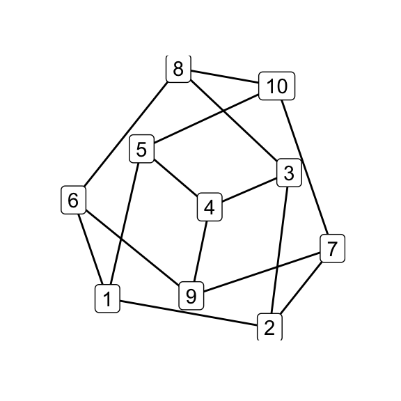
The Petersen family consists of seven graphs, up to isomorphism, that can be obtained from the original using so-called \(Y\)–\(\Delta\) and \(\Delta\)–\(Y\) operations.
\(Y\)–\(\Delta\) and \(\Delta\)–\(Y\)
Their names refer to the subgraphs that are exchanged in each operation, namely a 3-star (\(Y\)) and a 3-cycle (\(\Delta\)). The operations aren’t implemented in igraph, so here’s a clunky implementation usinng the R frontend:
# Y-Delta operations
wye_delta <- function(graph, v) {
  if (! all(degree(graph, v) == 3)) stop("Node(s) must have degree 3.")
  if (ecount(induced_subgraph(graph, v)) > 0) stop("Nodes cannot be adjacent.")
  nbhds <- mapply(setdiff, neighborhood(graph, 1, v), v)
  graph <- add_edges(graph, apply(nbhds, 2, combn, m = 2))
  graph <- delete_vertices(graph, v)
  graph
}
# Delta-Y operations
delta_wye <- function(graph, vt) {
  if (length(vt) %% 3 != 0) stop("Nodes must be triples.")
  if (is.matrix(vt) && nrow(vt) != 3) stop("Encode triples in matrix columns.")
  if (! is.matrix(vt)) vt <- matrix(vt, nrow = 3)
  tv <- vcount(graph) + 1:ncol(vt)
  graph <- add_vertices(graph, ncol(vt))
  graph <- add_edges(graph, rbind(as.vector(vt), rep(tv, each = 3)))
  graph <- delete_edges(graph, get.edge.ids(graph, apply(vt, 2, combn, m = 2)))
  graph
}
wye_delta() takes the vector of nodes v to be the centers of the 3-stars that will be converted to 3-cycles. These are required to have degree 3 and to be non-adjacent, so that there is no ambiguity when removing them. delta_wye() takes a vector or 3-row matrix of nodes vt that encode the 3-cycles. As with other igraph functions, these parameters will use numeric or character vectors as node IDs.
Petersen relations
To see how the Petersen family graphs are related by these operations, check out this preprint by O’Donnol. Viewing the Petersen family as a partially ordered set with respect to \(Y\)–\(\Delta\) and \(\Delta\)–\(Y\) operations, there are four extremal elements: the original Petersen graph and a graph named \(K_{4,4}\smallsetminus e\),4 which cannot be \(\Delta\)–\(Y\)’d (they have no 3-cycles), and the complete graph \(K_6\) and the complete tripartite graph \(K_{3,3,1}\), which cannot be \(Y\)–\(\Delta\)’d (without introducing multiple links).
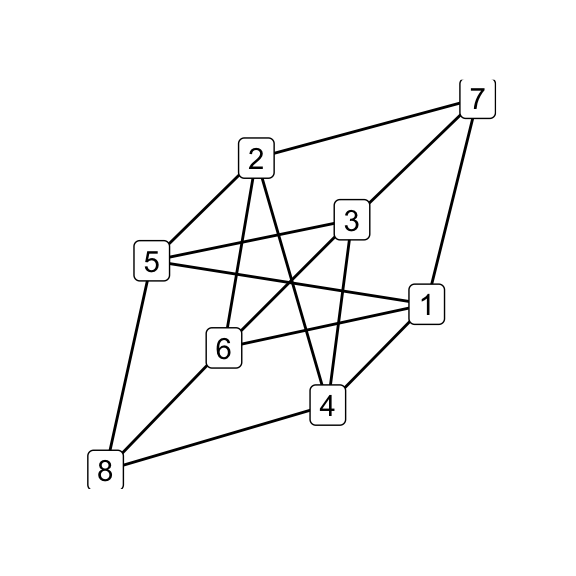
Following O’Donnol, and through some trial and error, i generated the Petersen family using the exchange operations, starting from \(K_6\) to get \(G_7\):
library(magrittr)
# complete graph on 6 nodes
make_full_graph(6) %T>% qgraph() -> k6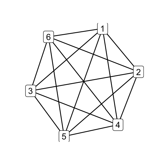
# G_7 via Delta-Y operation on K_6 at an arbitrary 3-cycle
delta_wye(k6, c(1,2,3)) %T>% qgraph() -> g7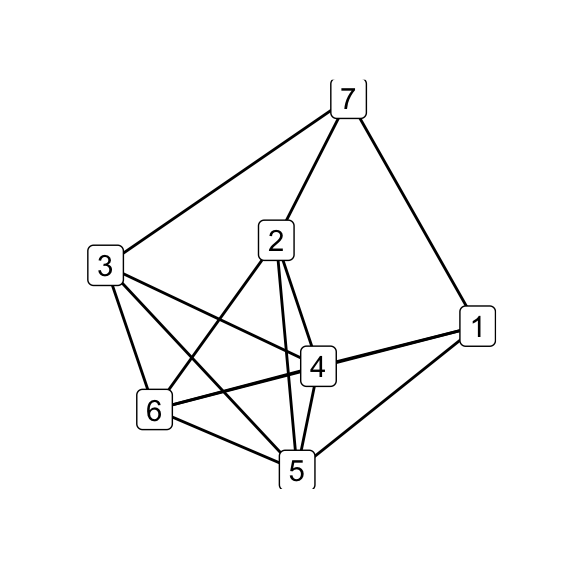
To illustrate how the simple relations among the family hinge on isomorphism classes, in the next step i perform all possible \(\Delta\)–\(Y\) operations on \(G_7\) and test the results for isomorphicity:
# all possible Delta-Y children
g7_children <- list(
  delta_wye(g7, c(1,4,5)),
  delta_wye(g7, c(2,4,5)),
  delta_wye(g7, c(3,4,5)),
  delta_wye(g7, c(3,4,6)),
  delta_wye(g7, c(3,5,6)),
  delta_wye(g7, c(4,5,6))
)
par(mfrow = c(2, 3))
for (i in seq_along(g7_children)) qgraph(g7_children[[i]])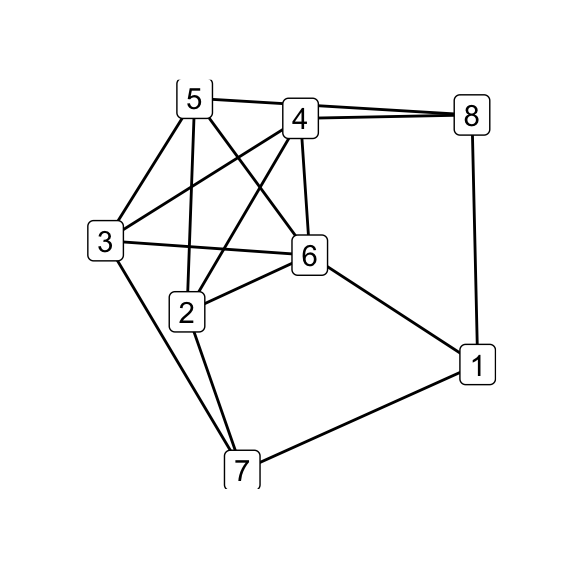
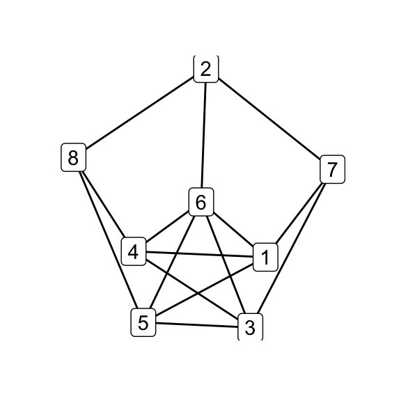
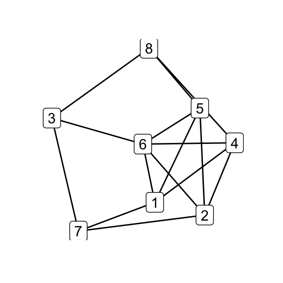
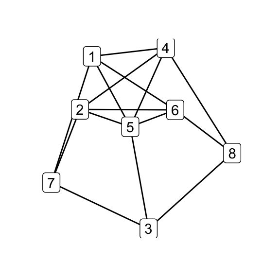
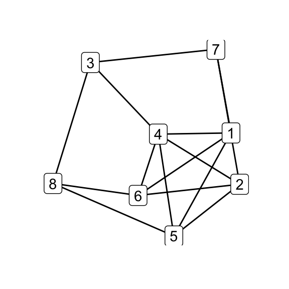
par(mfrow = c(1, 1))
# check which are isomorphic
isomat <- matrix(NA_integer_, nrow = 6, ncol = 6)
for (i in 1:5) for (j in (i+1):6) {
  isomat[i,j] <- isomat[j,i] <-
    as.integer(isomorphic(g7_children[[i]], g7_children[[j]]))
}
print(isomat)
## [,1] [,2] [,3] [,4] [,5] [,6]
## [1,] NA 1 1 1 1 0
## [2,] 1 NA 1 1 1 0
## [3,] 1 1 NA 1 1 0
## [4,] 1 1 1 NA 1 0
## [5,] 1 1 1 1 NA 0
## [6,] 0 0 0 0 0 NA# G_8 and K_44-e via Delta-Y operations on G_7
delta_wye(g7, c(3,4,5)) -> g8
delta_wye(g7, c(4,5,6)) -> k44_eOf the six possible \(\Delta\)–\(Y\) operations on \(G_7\), five produce \(G_8\) while one produces \(K_{4,4}\smallsetminus e\), indicating that the latter is in some sense less accessible than the former. Does that make \(K_{4,4}\smallsetminus e\), as its name would suggest, somehow less natural? Is the answer totally obvious to someone who’s absorbed the implications of embeddability as a theory, even if they haven’t directly observed the Petersen family before? (Does that even make sense?) Whether i come back to these questions is anyone’s guess.
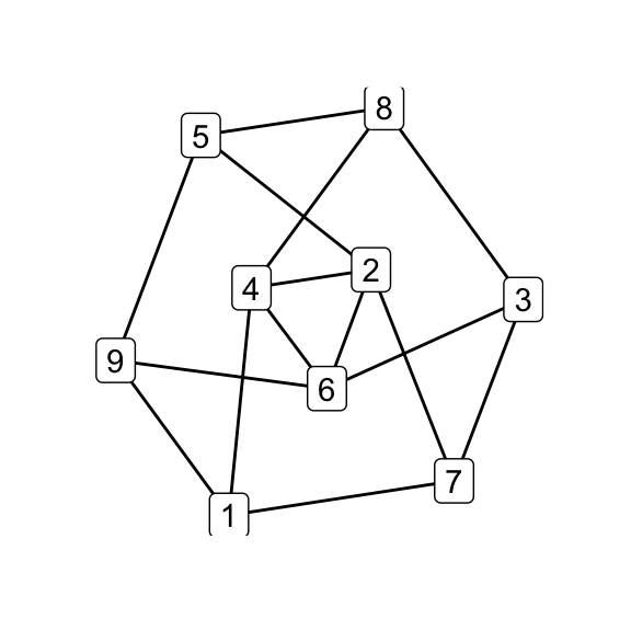
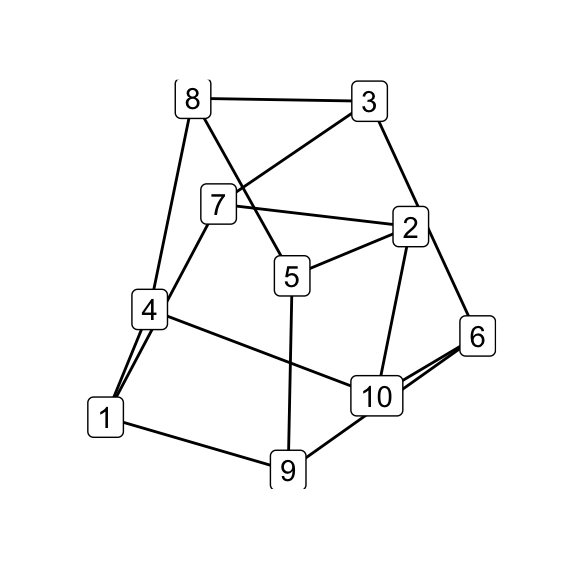
Anyway, the exchange operations can now take \(G_8\) up and down the rest of the poset, with a check at the end that we’ve arrived at the original Petersen graph. In these latter steps i’ve only presented one way to obtain each Petersen family member, but in each case there may be several.
# K_331 via Y-Delta operation on G_8
wye_delta(g8, 3) -> k331
# G_9 via Delta-Y operation on G_8
delta_wye(g8, c(1,5,6)) -> g9
# G_10 via Delta-Y operation on G_9
delta_wye(g9, c(2,4,6)) -> g10
par(mfrow = c(1, 3))
qgraph(k331); qgraph(g9); qgraph(g10)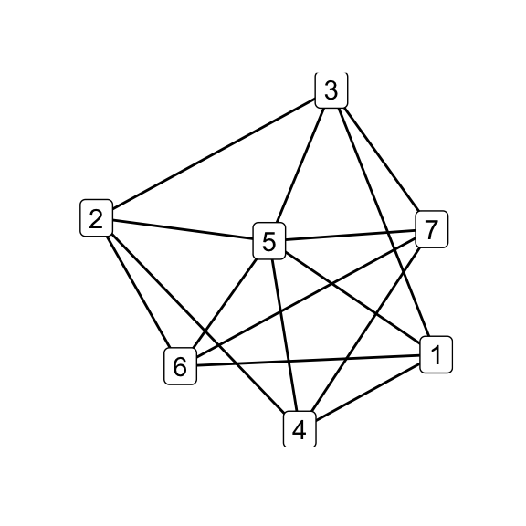
par(mfrow = c(1, 1))
# verify that G_10 is isomorphic to the Petersen graph
stopifnot(isomorphic(g10, petersen))
embeddings
Recall that the point of the Petersen family (for our purposes) is to encapsulate the constraints on linkless embeddability. To highlight this, i’d like to at least hint at how these constraints work by locating linked cycles in some very basic embeddings. I’ll start with the Petersen graph, using a Fruchterman–Reingold embedding as implemented in igraph:
library(dplyr)
library(tidyr)
library(plotly)
set.seed(0)
petersen %>%
  layout_with_fr(dim = 3) %>%
  as_tibble() %>%
  setNames(c("x", "y", "z")) %>%
  mutate(node = 1:nrow(.)) %>%
  print() -> nodes
## Warning: `as_tibble.matrix()` requires a matrix with column names or a `.name_repair` argument. Using compatibility `.name_repair`.
## This warning is displayed once per session.## # A tibble: 10 x 4
## x y z node
## <dbl> <dbl> <dbl> <int>
## 1 10.1 17.0 17.4 1
## 2 10.9 18.4 18.1 2
## 3 12.0 18.2 17.6 3
## 4 11.6 18.1 16.1 4
## 5 10.0 17.8 16.2 5
## 6 11.1 16.2 17.4 6
## 7 10.8 18.6 16.9 7
## 8 11.1 17.3 18.2 8
## 9 11.5 17.1 16.3 9
## 10 9.84 18.2 17.5 10coordinating z’s
Above, we produce a tibble of node coordinates. Below, we produce a tibble of link coordinates. This next chunk current complains and produces only a 2-dimensional visualization because plotly::add_segments() does not yet understand z-coordinates; i leave it here to return to as plotly continues to grow.
petersen %>%
  activate(links) %>%
  as_tibble() %>%
  left_join(nodes, by = c("from" = "node")) %>%
  left_join(nodes, by = c("to" = "node"), suffix = c("_from", "_to")) %>%
  print() -> links
## # A tibble: 15 x 8
## from to x_from y_from z_from x_to y_to z_to
## <int> <int> <dbl> <dbl> <dbl> <dbl> <dbl> <dbl>
## 1 1 2 10.1 17.0 17.4 10.9 18.4 18.1
## 2 1 5 10.1 17.0 17.4 10.0 17.8 16.2
## 3 1 6 10.1 17.0 17.4 11.1 16.2 17.4
## 4 2 3 10.9 18.4 18.1 12.0 18.2 17.6
## 5 2 7 10.9 18.4 18.1 10.8 18.6 16.9
## 6 3 4 12.0 18.2 17.6 11.6 18.1 16.1
## 7 3 8 12.0 18.2 17.6 11.1 17.3 18.2
## 8 4 5 11.6 18.1 16.1 10.0 17.8 16.2
## 9 4 9 11.6 18.1 16.1 11.5 17.1 16.3
## 10 5 10 10.0 17.8 16.2 9.84 18.2 17.5
## 11 6 8 11.1 16.2 17.4 11.1 17.3 18.2
## 12 6 9 11.1 16.2 17.4 11.5 17.1 16.3
## 13 7 9 10.8 18.6 16.9 11.5 17.1 16.3
## 14 7 10 10.8 18.6 16.9 9.84 18.2 17.5
## 15 8 10 11.1 17.3 18.2 9.84 18.2 17.5plot_ly(nodes, x = ~x, y = ~y, z = ~z) %>%
add_segments(
data = links,
x = ~x_from, xend = ~x_to,
y = ~y_from, yend = ~y_to,
z = ~z_from, zend = ~z_to,
color = I("black")
)## Warning: 'scatter' objects don't have these attributes: 'z', 'zend'
## Valid attributes include:
## 'type', 'visible', 'showlegend', 'legendgroup', 'opacity', 'name', 'uid', 'ids', 'customdata', 'selectedpoints', 'hoverinfo', 'hoverlabel', 'stream', 'transforms', 'uirevision', 'x', 'x0', 'dx', 'y', 'y0', 'dy', 'stackgroup', 'orientation', 'groupnorm', 'stackgaps', 'text', 'hovertext', 'mode', 'hoveron', 'hovertemplate', 'line', 'connectgaps', 'cliponaxis', 'fill', 'fillcolor', 'marker', 'selected', 'unselected', 'textposition', 'textfont', 'r', 't', 'error_x', 'error_y', 'xcalendar', 'ycalendar', 'xaxis', 'yaxis', 'idssrc', 'customdatasrc', 'hoverinfosrc', 'xsrc', 'ysrc', 'textsrc', 'hovertextsrc', 'hovertemplatesrc', 'textpositionsrc', 'rsrc', 'tsrc', 'key', 'set', 'frame', 'transforms', '_isNestedKey', '_isSimpleKey', '_isGraticule', '_bbox'The slightly more cumbersome solution is to organize the links as very short paths, distinguished by a grouping variable, in preparation for plotly::add_paths():
petersen %>%
  activate(links) %>%
  as_tibble() %>%
  mutate(link = row_number()) %>%
  gather(end, node, from, to) %>%
  left_join(nodes, by = "node") %>%
  group_by(link) %>%
  print() -> links
## # A tibble: 30 x 6
## # Groups: link [15]
## link end node x y z
## <int> <chr> <int> <dbl> <dbl> <dbl>
## 1 1 from 1 10.1 17.0 17.4
## 2 2 from 1 10.1 17.0 17.4
## 3 3 from 1 10.1 17.0 17.4
## 4 4 from 2 10.9 18.4 18.1
## 5 5 from 2 10.9 18.4 18.1
## 6 6 from 3 12.0 18.2 17.6
## 7 7 from 3 12.0 18.2 17.6
## 8 8 from 4 11.6 18.1 16.1
## 9 9 from 4 11.6 18.1 16.1
## 10 10 from 5 10.0 17.8 16.2
## # … with 20 more rowspl <- plot_ly(nodes, x = ~x, y = ~y, z = ~z)
pl <- add_paths(pl, data = links, x = ~x, y = ~y, z = ~z, color = I("black"))
pllinking cycles
Finally, a lucky guess hit upon two linked cycles in the above embedding, highlighted "firebrick" and "forestgreen" in the following 3-dimensional plot:
cycle1 <- 1:5
cycle2 <- c(6, 8, 10, 7, 9)
cycle1 %>%
  {get.edge.ids(petersen, rbind(., .[c(2:5, 1)]))} %>%
  tibble::enframe(name = NULL, value = "link") %>%
  inner_join(links, by = "link") ->
  cycle1
cycle2 %>%
  {get.edge.ids(petersen, rbind(., .[c(2:length(.), 1)]))} %>%
  tibble::enframe(name = NULL, value = "link") %>%
  inner_join(links, by = "link") -> cycle2
pl %>%
  add_paths(data = cycle1, x = ~x, y = ~y, z = ~z, color = I("firebrick")) %>%
  add_paths(data = cycle2, x = ~x, y = ~y, z = ~z, color = I("forestgreen")) %>%
  layout(showlegend = FALSE)
I’m happy to rest here, having figured out how to perform the famous embeddability-preserving operations and to render 3-dimensional graphics using plotly — which is about to become important as we prepare to present our anatomical analysis. If you take some further steps on your own, i’d be glad to hear about it!
I’m being carefully vague here while referring to possibly unpublished work.↩
I’m thinking here of consolidation as the mathematical analog of Mendeleev’s periodic table, which introduced a useful conceptual schema that was ultimately validated not by its elegance alone but by the brand new elements (pun) it implied For one of the best stories of consolodationist success in mathematics, read Baez’s popular chapter about the discoveries of the quarternions and the octonions leading up to the general Cayley–Dickson construction. A more recent example i’ve come to love is the modulus-based family of distance measures by Albin, Brunner, Perez, Poggi-Corradini, and Wiens that interpolate continuously between shortest path length and min flow–max cut distance.↩
I’m thinking of this “alignment” or “entanglement” to myself as the subspaces of the spaces of cycles of \(G\) and its complement, in the homological sense, having high-dimensional intersection, but that’s just a feeling.↩
I might call this graph “series–complete” on the ordered partition \((1,3,3,1)\), since the links are precisely the pairs of nodes in adjacent subsets. Probably graph theorists have a term for this.↩