Sampling uniformly from an embedded Klein bottle

an apparent dearth of toy TDA samplers

Experimenting and practicing with topological data analytic (TDA) tools requires a healthy diversity of suitable data sets. Several real-world classics can be found in various packages, for example the glucose and insulin test data collected and analyzed by Reaven and Miller and later used by Singh, Carlsson, and Mémoli to illustrate the Mapper construction, which is included in the heplots package:

data(Diabetes, package = "heplots")
head(Diabetes)

##   relwt glufast glutest instest sspg  group
## 1  0.81      80     356     124   55 Normal
## 2  0.95      97     289     117   76 Normal
## 3  0.94     105     319     143  105 Normal
## 4  1.04      90     356     199  108 Normal
## 5  1.00      90     323     240  143 Normal
## 6  0.76      86     381     157  165 Normal

For purposes of validation and comparison in particular, we need to supplement empirical data sets, which reflect potentially interesting but unknown topological structure, with artificial data sets that have known, and often simple, intrinsic topology. Probably the most commonly used are simulated samples from a circle, which are straightforward to generate in R:

library(magrittr)
library(tibble)
library(dplyr)
library(ggplot2)
tibble(theta = runif(120, 0, 2*pi)) %>%
  mutate(x = cos(theta), y = sin(theta)) %>%
  mutate_at(vars(x, y), funs(. + rnorm(n = length(.), sd = .1))) %>%
  print() %>%
  select(x, y) %>%
  ggplot(aes(x = x, y = y)) + coord_fixed() + geom_point()

## Warning: funs() is soft deprecated as of dplyr 0.8.0
## Please use a list of either functions or lambdas: 
## 
##   # Simple named list: 
##   list(mean = mean, median = median)
## 
##   # Auto named with `tibble::lst()`: 
##   tibble::lst(mean, median)
## 
##   # Using lambdas
##   list(~ mean(., trim = .2), ~ median(., na.rm = TRUE))
## This warning is displayed once per session.

## # A tibble: 120 x 3
##    theta      x      y
##    <dbl>  <dbl>  <dbl>
##  1 0.694  0.750  0.565
##  2 3.93  -0.662 -0.679
##  3 0.344  0.851  0.262
##  4 1.77  -0.308  1.06 
##  5 0.352  0.932  0.424
##  6 0.739  0.722  0.657
##  7 0.789  0.704  0.773
##  8 4.03  -0.713 -0.935
##  9 2.25  -0.459  0.806
## 10 0.742  0.745  0.703
## # … with 110 more rows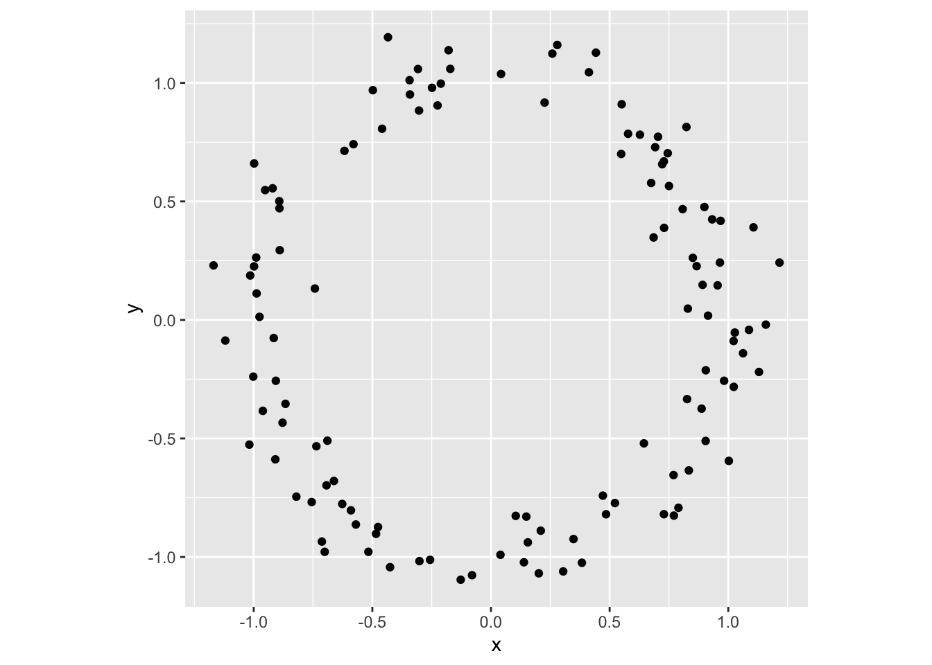

The underlying sampling protocol is, to my understanding, typical:¹

1. Pick a topological property to test for. In this case, most researchers want a loop, or a non-trivial generator in \(H_1(\,\cdot\,,\mathbb{Z})\).
2. Choose a manifold \(M\) having the desired property. The circle \(M=S^1\) is the simplest choice.
3. Choose a parameterization \(f:I\to M\subset\mathbb{R}^m\) from a parameter space \(I\) to an embedding of the manifold in an ambient Euclidean space. Most TDA actually depends on a data set having an underlying geometry, from which topological “nearness” is inferred. This choice determines that underlying geometry. Above, the parameter space is \([0,2\pi)\) and \(f(\theta)=(\cos(\theta),\sin(\theta))\).
4. Sample points \(S\subset M\) uniformly from the embedded manifold. The idea of uniformity makes sense because the manifold has a measure induced from the ambient space.
5. Optionally, add random noise to \(S\), usually from a standard \(m\)-dimensional Gaussian distribution.

While working with Raoul on the ggtda package, i’ve realized both how useful these simple artificial data sets are and how difficult they can be to find or produce. The TDA package can sample uniformly a sphere, and the KODAMA package can generate noisy spiral arrangements; but the most comprehensive sources i’ve found are the Python module TaDAsets, which includes three, and the Matlab toolbox drtoolbox, which includes seven. So, i’ve started accumulating “noisy shape” samplers into a lightweight R package that can be used as an alternative to saving specific samples for illustrative use in packages like ggtda. (If a better source exists that i haven’t found, please let me know!)

what else but a Klein bottle?

Naturally, the first thing i wanted to do was sample uniformly from a Klein bottle \(\mathbb{K}\). Parameterizations are easy to find, e.g. on Wikipedia, and i opted for one that looked most similar to the usual “doughnut” parameterization of the torus in \(\mathbb{R}^3\), namely the “Möbius tube” in \(\mathbb{R}^4\):

\[\begin{align*} w(\theta,\phi) &= (1 + r\cos\theta)\cos\phi \\ x(\theta,\phi) &= (1 + r\cos\theta)\sin\phi \\ y(\theta,\phi) &= r\sin\theta\cos\frac{\phi}{2} \\ z(\theta,\phi) &= r\sin\theta\sin\frac{\phi}{2} \end{align*}\]

The parameter space is \([0,2\pi)\times[0,2\pi)\ni(\theta,\phi)\), while \(r\) is a constant that determines the shape of the embedded manifold. (Here i’ve simplified the Wikipedia parameterization by setting \(R=1\) and assuming that \(0\leq r\leq 1\).) So here’s a closure that takes r as input and returns a parameterization function that sends a data frame of \(\theta,\phi\) coordinates to one of \((w,x,y,z)\) coordinates:

param_klein <- function(r) {
  if (r < 0 | r > 1) stop("`r` must be between 0 and 1.")
  function(data) {
    with(data, tibble(
      w = (1 + r * cos(theta)) * cos(phi),
      x = (1 + r * cos(theta)) * sin(phi),
      y = r * sin(theta) * cos(phi / 2),
      z = r * sin(theta) * sin(phi / 2)
    ))
  }
}

Sampling is another matter. Though we know the embedding warps the parameter space, stretching parts of it while compressing others, it’s tempting to presuppose that this warping will not vary too much, and just take uniform samples from the parameter space and map them to the ambient space. Here’s where that gets us, without adding additional noise:

f_klein <- param_klein(r = .75)
tibble(theta = runif(360, 0, 2*pi), phi = runif(360, 0, 2*pi)) %>%
  f_klein() %>%
  print() %>%
  pairs(asp = 1, pch = 19, cex = .5, col = "#00000077")

## # A tibble: 360 x 4
##          w      x       y       z
##      <dbl>  <dbl>   <dbl>   <dbl>
##  1  0.300   0.938  0.606   0.442 
##  2 -0.191   0.172  0.0377  0.0983
##  3  1.69    0.296  0.238   0.0208
##  4  0.0991  1.14  -0.542  -0.497 
##  5  0.714  -0.678  0.696  -0.278 
##  6 -0.340  -0.372 -0.227   0.514 
##  7 -0.471   0.987  0.397   0.629 
##  8  0.465   1.17   0.583   0.395 
##  9  0.495  -0.405  0.619  -0.221 
## 10  0.155   0.226  0.166   0.0874
## # … with 350 more rows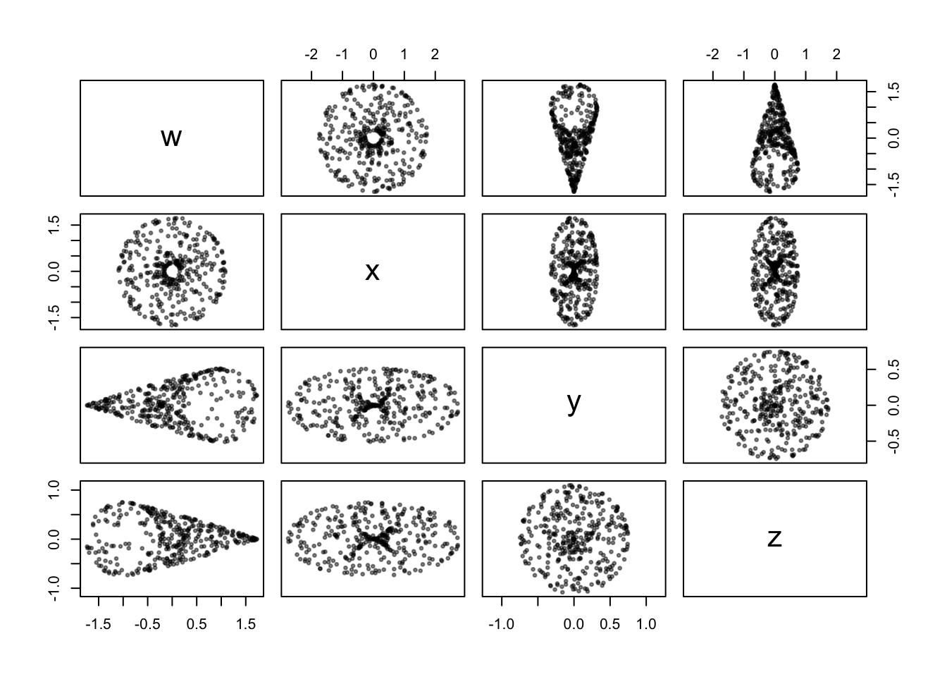

The features of the manifold are recognizable: The projection onto \(w\) and \(x\) is like that of a torus, while complementary “pinches” are discernible in the \(y\) and \(z\) directions with respect to \(w\). However, it’s also clear that more points have been sampled toward the center of the shape, where the parameterization “moves” most slowly, while fewer have been sampled toward the periphery. While we can visually pick out other regions of higher and lower concentrations, it’s not obvious how to determine how much of this is due to warping by the parameterization versus the angle from which we’re viewing the sample in these scatterplots.

point cloud topology is sensitive to geometry

To better illustrate the potential problem, let’s go back to the noisy circle. The standard parameterization has the very nice property that the rate at which \(f(\theta)\) traverses the circle, with respect to the rate at which \(\theta\) proceeds along the interval, is constant. In analytic terms, the gradient \(\nabla f=(\frac{\partial x}{\partial\theta},\frac{\partial y}{\partial\theta})\) has constant magnitude. Instead of this standard, consider the alternative, highly suspect parameterization \(g:[-2,2)\to\mathbb{R}^2\) given by

\[g(t) = \begin{cases} (t+1,\sqrt{1-(t+1)^2}) & t\leq 0 \\ (1-t,-\sqrt{1-(1-t)^2}) & t>0 \end{cases}\]

This map takes the interval \([-2,0]\), shifts it rightward to \([-1,1]\), and lifts it to the upper hemicircle; to complement, it shifts \(0,2\) leftward to \((-1,1)\), reverses it (so that the map is continuous at \(t=0\)), and drops it to the lower hemicircle. Here’s how the sampling procedure shakes out:

tibble(t = runif(120, -2, 2)) %>%
  mutate(x = ifelse(t <= 0, t + 1, 1 - t)) %>%
  mutate(y = ifelse(t <= 0, sqrt(1 - x^2), -sqrt(1 - x^2))) %>%
  mutate_at(vars(x, y), funs(. + rnorm(n = length(.), sd = .1))) %>%
  select(x, y) %>%
  ggplot(aes(x = x, y = y)) + coord_fixed() + geom_point()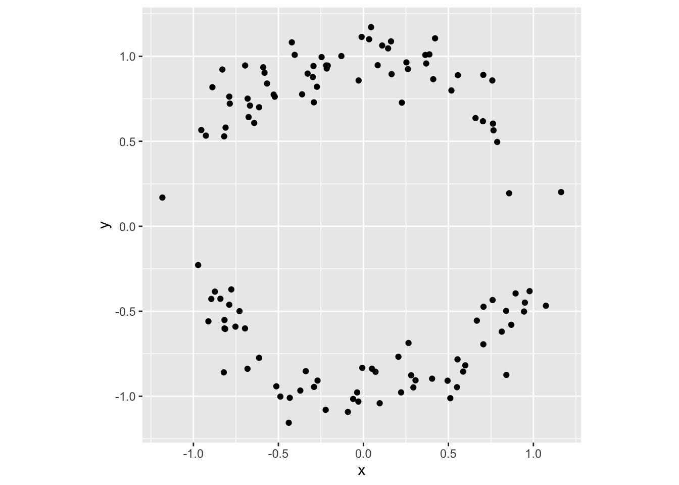

Notice the sparsity of points near \((-1,0)\) and \((1,0)\). This is because, as \(x(t)\) moves steadily away from these endpoints, \(y(t)\) bolts away from them; so that the Euclidean distance \(\sqrt{x^2+y^2}\) between \(g(t_0)\) and \(g(t_1)\) is larger when \(t_0\) and \(t_1\) are closer to these endpoints than when they are closer to \((0,1)\) or \((0,-1)\). This is the sort of problem we want to be sure to avoid when sampling from the embedded Klein bottle.

reforming a deformed sampler

My solution comes from a very cool paper titled “Sampling from a Manifold”, by mathematicians Persi Diaconis and Mehrdad Shahshahani and statistician Susan Holmes. I don’t remember how i first came across this paper, but i found it simultaneously exciting and exhausting to read — excited by the prospect of using basic calculus and computational trickery to generate uniform manifold samples, exhausted by the way rigorous details were either compactified or outsourced. This post was ultimately motivated by a desire, for my own future benefit at least, to have a thoroughly documented application of their method available for reference.

Recall the Möbius tube parameterization \(f:[0,2\pi)\times[0,2\pi)\to\mathbb{R}^4\) above. To correct for the warping \(f\) introduces, the strategy is to measure this warping locally (i.e. as a function of the parameters \(\theta\) and \(\phi\)) and then filter our random samples in a way that undoes its effects.

vector derivatives

As i alluded in the example of the circle, the warping arises from differences in the rate at which distances in the domain \(I\subset\mathbb{R}^2\) translate into distances in the codomain \(\mathbb{R}^4\). That is to say, we measure the warping in terms of derivatives. The vector-valued function \(f\) has two inputs and four outputs, so its \(4\times 2\) Jacobian (derivative) matrix \(J_f\) is given by

\[J_f= \left[\ \frac{\partial f}{\partial\theta}\ \frac{\partial f}{\partial\phi}\ \right]= \left[\begin{array}{cc} \frac{\partial w}{\partial\theta} & \frac{\partial w}{\partial\phi} \\ \frac{\partial x}{\partial\theta} & \frac{\partial x}{\partial\phi} \\ \frac{\partial y}{\partial\theta} & \frac{\partial y}{\partial\phi} \\ \frac{\partial z}{\partial\theta} & \frac{\partial z}{\partial\phi} \end{array}\right]= \left[\begin{array}{cc} -r\sin\theta\cos\phi & -(1+r\cos\theta)\sin\phi \\ -r\sin\theta\sin\phi & (1+r\cos\theta)\cos\phi \\ r\cos\theta\cos\frac{\phi}{2} & -\frac{1}{2}r\sin\theta\sin\frac{\phi}{2} \\ r\cos\theta\sin\frac{\phi}{2} & \frac{1}{2}r\sin\theta\cos\frac{\phi}{2} \end{array}\right]\]

Locally, the domain is composed of rectangles \((\theta,\theta+\Delta\theta)\times(\phi,\phi+\Delta\phi)\), while the codomain is, up to linear approximation, composed of parallelograms \((f,f+\frac{\partial f}{\partial\theta}\Delta\theta,f+\frac{\partial f}{\partial\phi}\Delta\phi,f+\frac{\partial f}{\partial\theta}\Delta\theta+\frac{\partial f}{\partial\phi}\Delta\phi)\). Whereas the domain rectangles have area \(\Delta\theta\Delta\phi\), the codomain parallelograms have area \(\Delta A=(\lvert\frac{\partial f}{\partial\theta}\rvert\lvert\frac{\partial f}{\partial\phi}\rvert\cos\omega)\Delta\theta\Delta\phi\), where \(\omega\) is the angle between the vectors \(\frac{\partial f}{\partial\theta}\) and \(\frac{\partial f}{\partial\phi}\). The local area function is then \(\lvert\frac{\partial f}{\partial\theta}\rvert\lvert\frac{\partial f}{\partial\phi}\rvert\cos\omega\).

The more elegant way to understand this² is by imagining that \(f\) takes a space, say \(\mathbb{R}^2\), to itself. In this case, the matrix \(J_f=\left[\ \frac{\partial f}{\partial\theta}\ \frac{\partial f}{\partial\phi}\ \right]\) consists of the two (column) vectors in \(\mathbb{R}^2\) defining the parallelogram corresponding to the unit rectangle based at \((\theta,\phi)\in\mathbb{R}^2\), so that the area of the parallelogram is the absolute value of \(\det J_f\). This generalizes to the formula \(j_f=\sqrt{\det({J_f}^\top{J_f})}\) when the domain and codomain have different dimensions.

A bit of algebra (minus the frustrating hours i lost after forgetting to differentiate constants) yields the Jacobian determinant \[j_f = r\sqrt{(1+r\cos\theta)^2 + (\frac{1}{2}r\sin\theta)^2}\text.\] As before, the function is returned from a closure that depends on r:

jacobian_klein <- function(r) {
  function(theta) r * sqrt((1 + r * cos(theta)) ^ 2 + (.5 * r * sin(theta)) ^ 2)
}

Here’s how the Jacobian determinant — that is, the expanding and contracting of area by the parameterization — depends on \(\theta\):

j_klein <- jacobian_klein(r = .75)
tibble(theta = seq(0, 2*pi, length.out = 60)) %>%
  mutate(jacobian = j_klein(theta)) %>%
  print() %>%
  ggplot(aes(x = theta, y = jacobian)) +
  ylim(c(0, NA)) +
  geom_line() +
  geom_area(fill = "#00000077")

## # A tibble: 60 x 2
##    theta jacobian
##    <dbl>    <dbl>
##  1 0         1.31
##  2 0.106     1.31
##  3 0.213     1.30
##  4 0.319     1.29
##  5 0.426     1.27
##  6 0.532     1.24
##  7 0.639     1.21
##  8 0.745     1.18
##  9 0.852     1.14
## 10 0.958     1.10
## # … with 50 more rows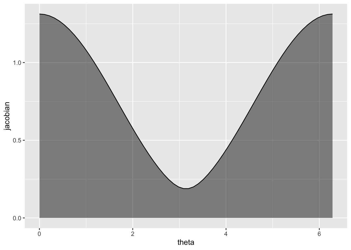

Looking back at the scatterplots, the contraction is least near \(\theta=0\) and \(\theta=2\pi\), toward the periphery of the Klein bottle where \(w\) and \(x\) are at their greatest amplitudes (with respect to \(\phi\)), and greatest near \(\theta=\pi\), toward the center.

de-biasing samples

We can now use our knowledge of derivatives to preempt the bias they introduce. The motivation is that, if the surface is expanded by a factor of \(k\) near the point \((\theta_0,\phi_0)\), then \(k\) times as many points should be sampled there, so that the density of points on the warped surface is uniform. The idea of rejection sampling, with a density function \(\delta:I\to[0,1]\), is to sample many points uniformly and then retain each point \((\theta_0,\phi_0)\) with probability \(\delta(\theta_0,\phi_0)\).

In fact, we don’t have to calculate the density function exactly, so that it has unit integral over the domain \(I\); it is enough to make sure that we retain samples in the correct proportion. Since the Jacobian is maximized at \(\theta=0\) for any choice of \(r\),³ this can be accomplished as follows:

1. Sample \(\theta\in[0,2\pi)\) uniformly.
2. Sample \(\eta\in[0,j_f(0)]\) uniformly.
3. If \(j_f(\theta) > \eta\), then retain the value \(\theta\); otherwise, reject \(\theta\).

Effectively, we retain \(\theta\) when \((\theta,\eta)\) lies in the shaded region above and reject it when not. The procedure repeats until enough values are retained. This leads me to the following rejection sampler:

sample_klein_theta <- function(n, r) {
  x <- c()
  while (length(x) < n) {
    theta <- runif(n, 0, 2 * pi)
    jacobian <- jacobian_klein(r)
    jacobian_theta <- sapply(theta, jacobian)
    eta <- runif(n, 0, jacobian(0))
    x <- c(x, theta[jacobian_theta > eta])
  }
  x[1:n]
}
sample_klein <- function(n, r) {
  d <- tibble(
    phi = runif(n, 0, 2*pi),
    theta = sample_klein_theta(n, r)
  )
  f <- param_klein(r)
  f(d)
}

We can compare this to the naïve sampler above that did not account for warping by the parameterization:

sample_klein(n = 360, r = .75) %>%
  print() %>%
  pairs(asp = 1, pch = 19, cex = .5, col = "#00000077")

## # A tibble: 360 x 4
##          w      x       y       z
##      <dbl>  <dbl>   <dbl>   <dbl>
##  1  1.59   -0.326  0.411  -0.0417
##  2 -0.0144  0.459 -0.362  -0.373 
##  3 -0.853   1.12  -0.280  -0.565 
##  4 -1.66    0.243 -0.0237 -0.326 
##  5 -1.43    0.712 -0.105  -0.446 
##  6  1.19    0.595 -0.654  -0.154 
##  7  0.222  -0.506  0.504  -0.329 
##  8  1.32   -0.334  0.654  -0.0818
##  9  0.861   0.361 -0.732  -0.147 
## 10  0.0688  1.22  -0.521  -0.492 
## # … with 350 more rows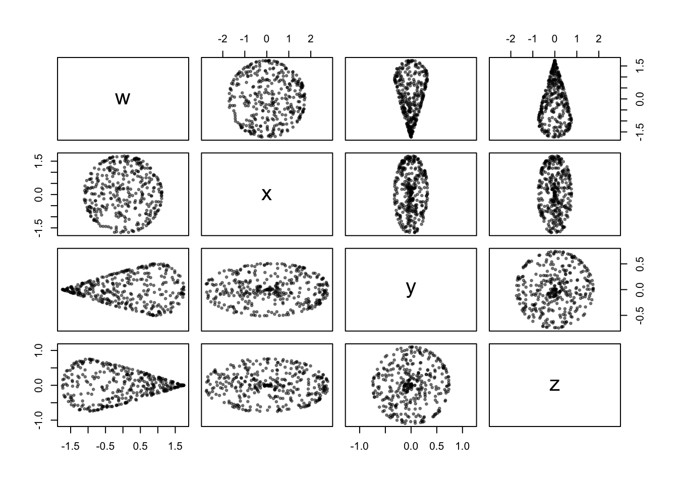

The differences are minor in most of the coordinate scatterplots, but the concentration of points near the center of the \(w,x\)-projection is clearly less than before, and not discernibly different at this “inner” region of the surface than at the “outer” regions.

validation via persistent homology

It makes sense to wrap up with a validation test. In an inversion of the usual protocol, i’ll use a widely-used implementation of persistent homology (PH) to validate my sampler. Since PH is based on distances in the ambient space \(\mathbb{R}^4\), the topological features of the Klein bottle — two generators of the rank-1 homology group \(H_1(\mathbb{K},\mathbb{Z})\) — should be more clearly discernible from the points sampled uniformly from the embedded manifold than from those embedded from a uniform sample on the parameter space. In order to better illustrate the limiting case, i’ve boosted the sample size to 840 and set the minor radius to half the major radius. Here are the persistence diagrams for both samples:

f_klein <- param_klein(r = .5)
tibble(theta = runif(840, 0, 2*pi), phi = runif(840, 0, 2*pi)) %>%
  f_klein() %>%
  as.matrix() %>%
  TDAstats::calculate_homology(dim = 1) %>%
  TDAstats::plot_persist() +
  scale_y_continuous(limits = c(0, 1)) ->
  ph_klein_warp
sample_klein(n = 840, r = .5) %>%
  as.matrix() %>%
  TDAstats::calculate_homology(dim = 1) %>%
  TDAstats::plot_persist() +
  scale_y_continuous(limits = c(0, 1)) ->
  ph_klein_unif
gridExtra::grid.arrange(ph_klein_warp, ph_klein_unif, ncol = 2)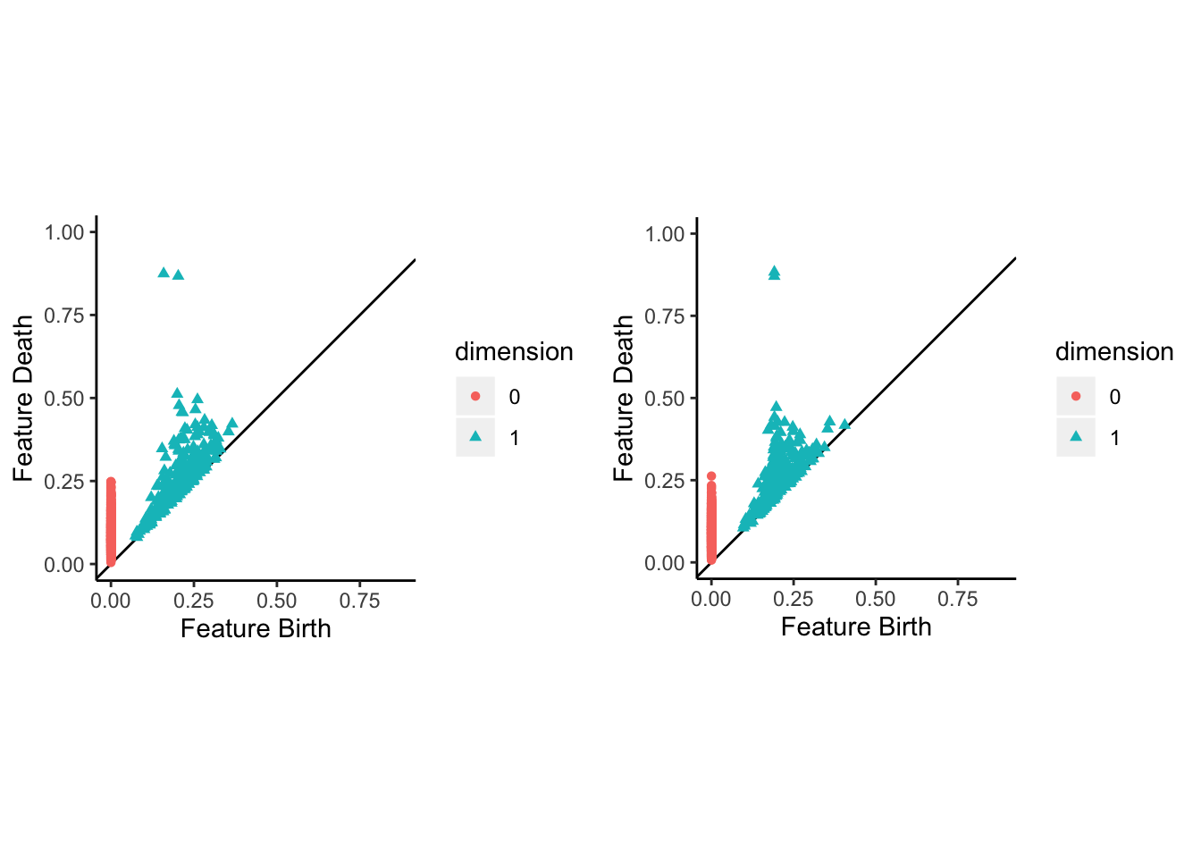

Indeed, while PH captures the topology of \(\mathbb{K}\) from both samples, the noise is noticeably reduced in the latter. Voila!⁴